October 10, 2026

⛶

What this problem really is

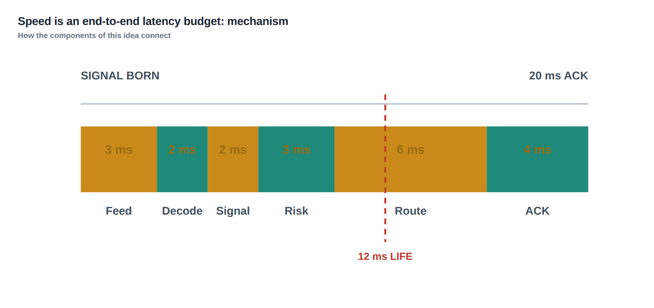
The latency budget of an electronic strategy is not a single number that can be quoted in a brochure; it is the sum of every interval that lies between the instant a market data packet arrives at the gateway and the moment the exchange acknowledges the execution of the order that was generated from that packet. In a price‑time‑priority market each millisecond that a trader spends waiting for a decision is a millisecond in which the queue position may slip, the spread may narrow and the adverse‑selection risk may increase. Consequently the “speed” of a strategy is bounded by the slowest useful stage in that end‑to‑end chain, not by the fastest component.

If the market moves faster than the slowest stage, the information that triggered the signal will have decayed, and the order will be submitted into a queue that no longer offers the expected profit. The problem therefore becomes one of budgeting: how much time can be allocated to feed handling, to decoding, to signal computation, to risk checks, to routing, and finally to acknowledgement, before the economic half‑life of the signal has elapsed? The answer is a function of the instrument’s micro‑structure, of the venue’s latency characteristics, and of the strategy’s own statistical decay profile.

A naïve latency optimisation that focuses only on the fastest path through a single server will ignore the fact that the market’s own dynamics impose a hard deadline on the usefulness of any piece of information. The “fastest possible” number is therefore irrelevant unless it is compared with the signal’s half‑life and with the total decision‑to‑acknowledgement latency that the system actually experiences in production.

—

How the mechanism works, step by step

The first stage is the physical transmission of market data from the exchange’s matching engine to the trader’s gateway. This feed transit time is a function of network topology, fibre length, and any intermediate switches; it can be measured in sub‑microseconds on a dedicated line but may rise to several hundred microseconds on a public Internet route.

Once the packet reaches the gateway it must be deserialised and transformed into an internal representation. Decoding latency is often overlooked because modern parsers are highly optimised, yet the cumulative effect of checksum verification, protocol conversion and timestamp normalisation can add a measurable jitter component, especially under high‑throughput conditions.

The decoded data then enters the signal engine. Here the algorithm evaluates the market snapshot against its statistical model and produces a trade intent. The calculation itself may be trivial (a few arithmetic operations) or complex (machine‑learning inference). In the worked example the signal calculation consumes two milliseconds, a figure that seems modest but becomes critical when the downstream path is much longer.

Risk checks follow immediately. They verify position limits, margin requirements, and compliance constraints. Because these checks must be performed on the same data that generated the signal, any delay here directly eats into the remaining latency budget. In practice risk checks can be parallelised, but the coordination overhead introduces its own tail latency.

Routing is the act of selecting the optimal outbound path to the destination venue. Modern smart‑order routers evaluate multiple routes, apply cost models and possibly fragment the order. The routing decision is therefore not instantaneous; a well‑designed router may spend a few hundred microseconds, but under stress this can swell to several milliseconds.

Finally the order reaches the exchange gateway, where it is placed into the order book and an acknowledgement is sent back. The acknowledgement latency is the only part of the chain that is visible to the trader as a round‑trip time, yet it includes all the previous stages. If the total decision‑to‑acknowledgement latency exceeds the economic half‑life of the signal, the trade will be executed on stale information.

—

A worked example with real numbers

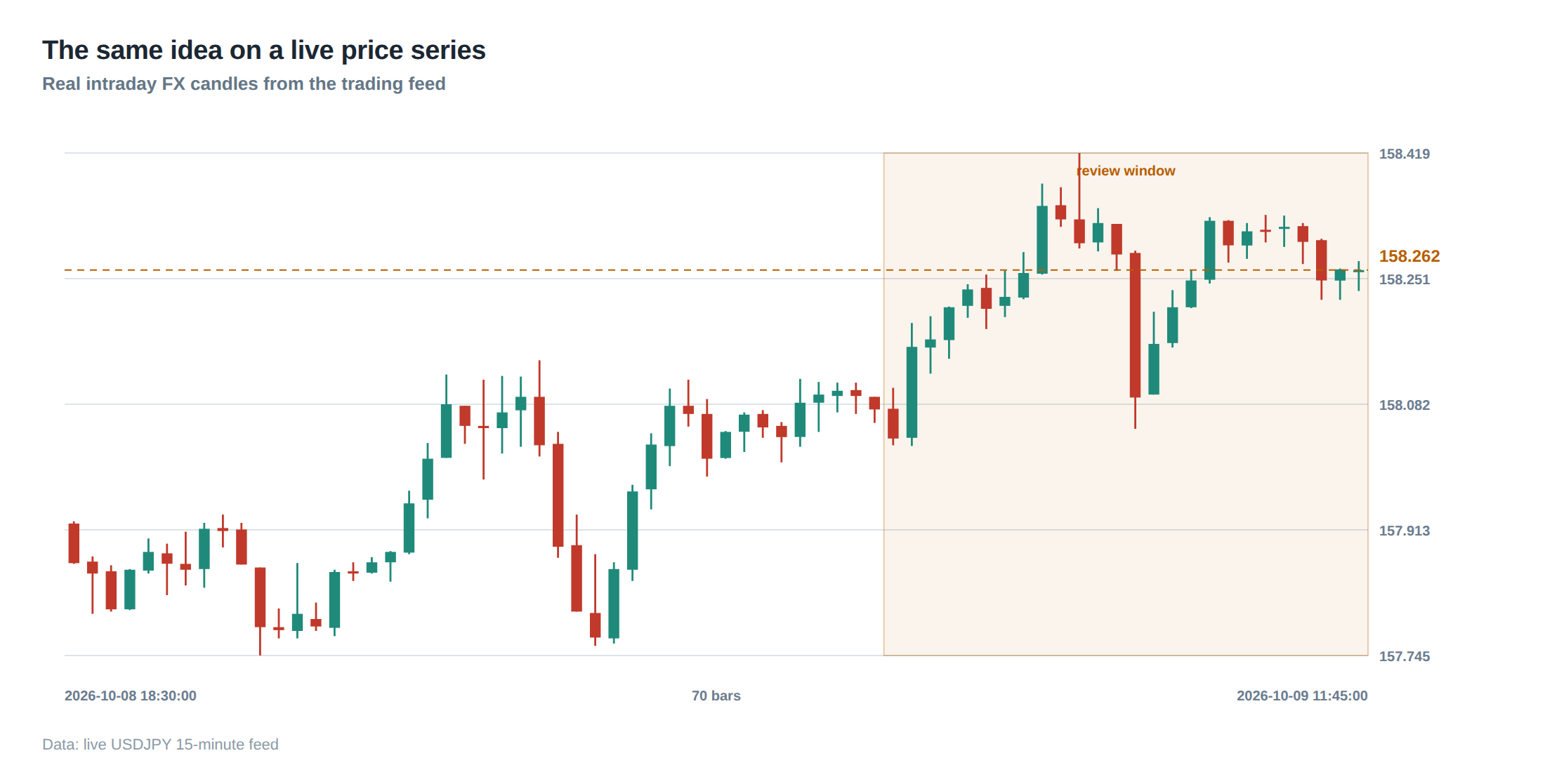
Consider a high‑frequency market‑making strategy that targets a 0.5 % spread on a liquid equity. Empirical analysis shows that the expected profit from a favourable price move decays with a half‑life of roughly twelve milliseconds; after that the probability of capturing the spread falls below 50 %. The signal engine, running a simple micro‑price imbalance model, takes two milliseconds to produce a trade intent.

The feed transit from the exchange to the co‑located gateway is measured at 0.8 ms median, with a 99th‑percentile of 1.4 ms. Decoding adds 0.4 ms median and a tail of 0.9 ms. Risk checks consume 0.6 ms on average, while the smart‑order router spends 1.2 ms median but can reach 3 ms in the tail. The exchange’s acknowledgement latency is 1.0 ms median, 2.5 ms at the 99th percentile.

Summing the medians yields a total decision‑to‑acknowledgement latency of 5.0 ms, comfortably below the twelve‑millisecond half‑life. However, when we consider the tail values – 1.4 + 0.9 + 0.6 + 3.0 + 2.5 = 8.4 ms – the total approaches the half‑life, leaving little margin for unexpected queuing delays on the exchange side. If the order path ever expands to twenty milliseconds, as can happen during a burst of market activity, the two‑millisecond signal calculation becomes essentially useless; the opportunity will have vanished long before the order can be placed.

The example therefore illustrates the core thesis: a fast signal is of limited value if the downstream latency budget is not proportionally small, and the tail behaviour of each stage is as important as the median.

—

Where it breaks in live markets

In live trading the latency budget is constantly challenged by external factors that are not under the trader’s control. Sudden spikes in network congestion can increase feed transit by a factor of two, while hardware throttling due to thermal limits can add microseconds of decoding jitter. More pernicious is the phenomenon of “queue creep” on the exchange: as other participants submit orders, the position of a newly submitted order can be displaced within the price‑time queue, effectively reducing the remaining time to capture the spread.

When the market experiences a rapid price swing, the signal’s half‑life can contract dramatically. A move that would normally decay over twelve milliseconds may become irrelevant after six milliseconds if volatility spikes. In such regimes the tail latency of any stage becomes a liability; a single outlier in routing time can cause the whole order to miss the price window.

Another failure mode is timestamp misalignment. If the exchange’s timestamps are not synchronised with the trader’s clock, the measured latency may be understated, leading to an illusion of speed that does not translate into economic advantage. In practice, clock drift of even a few microseconds can distort the perceived order‑to‑acknowledgement time, especially when the strategy relies on sub‑microsecond decision thresholds.

Finally, the assumption that an order’s lifetime can be expressed purely as elapsed wall‑clock time is flawed. The research on price‑time‑priority queues shows that the value of staying in line is a function of the expected spread, the adverse‑selection risk, and the option value of retaining a queue position. When market conditions change, the optimal decision may be to cancel an order early, even if the wall‑clock budget has not been exhausted.

—

The operating path, stage by stage

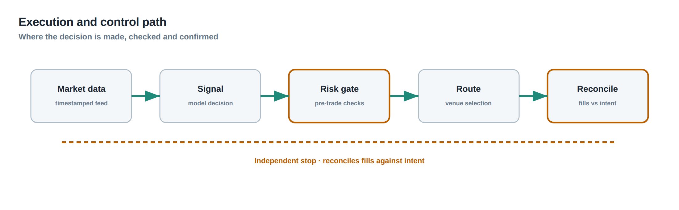
Feed transit is the first gatekeeper. To keep this stage within a tight budget, firms co‑locate their gateway hardware inside the exchange’s data centre and employ low‑latency fibre or microwave links. The physical distance is measured in metres, and even a ten‑metre increase can add a nanosecond of propagation delay, which is material when the total budget is measured in single‑digit milliseconds.

Decoding follows, and the choice of protocol (FIX, ITCH, proprietary binary) dictates the parsing complexity. A well‑engineered decoder will use zero‑copy techniques and SIMD instructions to keep the per‑packet processing time below one microsecond. Nevertheless, the variance introduced by packet reordering or occasional checksum failures can generate jitter that must be accounted for in the latency distribution.

Signal calculation is the intellectual core. Whether the model is a linear regression or a deep‑neural network, the implementation must be profiled to guarantee that the worst‑case execution time does not exceed a fraction of the signal’s half‑life. Techniques such as model quantisation, pre‑fetching of market data, and lock‑free data structures are common ways to shave off microseconds.

Risk checks are often the most mutable stage, as they depend on the current portfolio state. By maintaining a real‑time view of exposures in shared memory and by using atomic operations, the system can keep the risk‑check latency deterministic. However, any additional compliance rule that is introduced later will inevitably add to the path.

Routing is where the order is matched to an outbound channel. Modern smart‑order routers maintain a live cost table for each venue, updating it with market‑impact estimates and fee structures. The router must therefore perform a small optimisation problem for every order. By limiting the candidate set to a few venues and by pre‑computing the cost surface, the router can stay within a few hundred microseconds.

Acknowledgement is the final feedback loop. The exchange’s acknowledgement timestamp is the only reliable external marker of when the order entered the book. To close the loop, the trader’s system must correlate this timestamp with the original market‑data timestamp, correcting for any clock offset. The resulting round‑trip latency is the metric that drives the end‑to‑end budget.

—

Controls that act before the damage

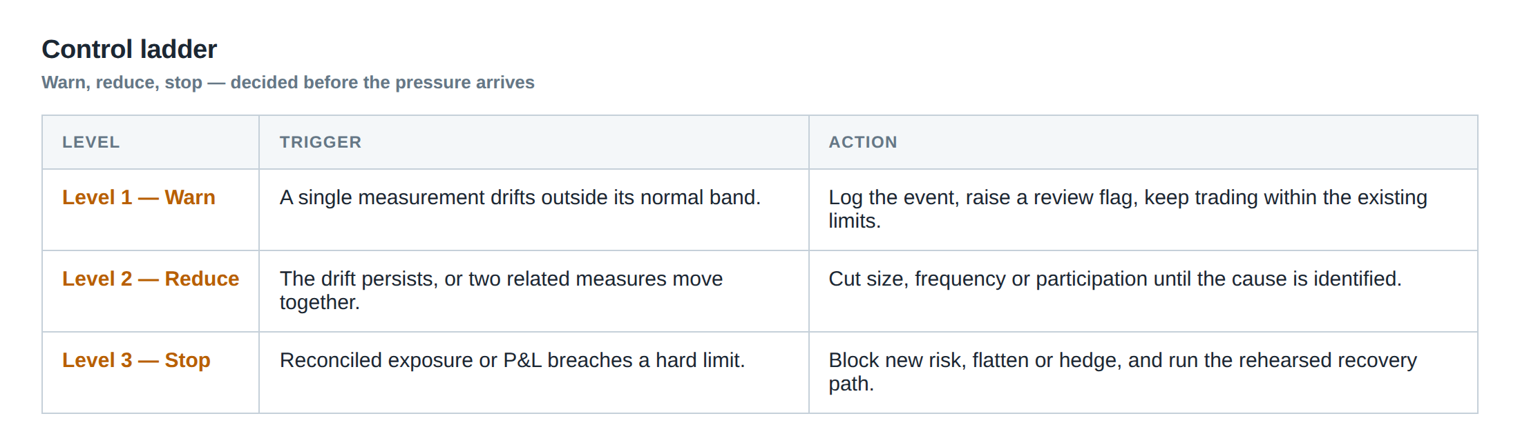
Pre‑emptive controls are essential because once an order is in the exchange’s queue the trader has lost the ability to influence its fate without incurring additional latency. One control is the “latency guardrail”: the system continuously monitors the median and tail latencies of each stage and, if a threshold is breached, automatically disables the strategy or switches to a slower, more robust mode.

Another safeguard is the dynamic half‑life estimator. By analysing recent price‑impact curves, the platform can adjust the acceptable latency budget in real time. If volatility rises and the half‑life contracts, the estimator will tighten the guardrail, forcing the signal engine to either speed up or suppress trading until conditions stabilise.

Clock synchronisation is treated as a control rather than a measurement artefact. The system employs a disciplined time protocol such as PTP (Precision Time Protocol) with hardware timestamping, and it continuously validates the offset against the exchange’s reference clock. Any drift beyond a few microseconds triggers an alarm and forces the latency measurements to be discarded until the clock is re‑aligned.

Finally, a “queue‑value monitor” evaluates the expected profit of staying in line versus cancelling. It uses the current spread, the depth of the order book, and the estimated adverse‑selection probability to decide whether to let the order sit for the full latency budget or to pull it early. This decision is made before the order reaches the exchange, thereby avoiding wasteful exposure to stale queue positions.

—

How to measure whether it is working

Measurement must be performed on the same data path that the strategy uses in production; synthetic benchmarks that bypass the network or the decoder give a false sense of speed. The primary metric is the distribution of end‑to‑end latency, expressed as median, 95th‑percentile, and 99th‑percentile values. Jitter is quantified by the inter‑quartile range of the latency distribution.

Each stage should be instrumented with high‑resolution timestamps taken as close as possible to the physical event (e.g., at the NIC for feed arrival, at the decoder entry point, after the signal engine, after risk checks, at the router output, and at the acknowledgement receipt). The timestamps must be synchronised to a common clock, otherwise the summed latency will be polluted by clock skew.

A useful sanity check is to compare the measured signal half‑life with the observed decision‑to‑acknowledgement latency. If the 99th‑percentile latency exceeds the half‑life, the strategy is effectively trading on stale signals. In that case the control system should either tighten the latency guardrail or adjust the model to produce longer‑lasting signals.

Continuous monitoring dashboards should display not only the latency percentiles but also the correlation between latency spikes and profit‑and‑loss drift. A rise in tail latency that coincides with a drop in realised spread capture is a strong indicator that the latency budget is being violated in a way that harms performance.

—

The portfolio view

From a portfolio perspective, latency is an invisible cost that manifests as reduced fill probability, higher adverse‑selection loss, and diminished spread capture. When the latency budget is respected, the strategy’s edge can be modelled as a deterministic component that adds a fixed percentage to the Sharpe ratio. When the budget is breached, the edge becomes stochastic, and the portfolio’s variance inflates.

The end‑to‑end latency budget also interacts with capital allocation. A strategy that operates near the latency limit may require a larger capital cushion to survive occasional tail events, because a missed opportunity does not just forego profit but also leaves the position exposed to market moves that the model could not hedge in time.

Risk‑adjusted performance metrics such as the information ratio should therefore be computed on a latency‑filtered data set: only those trades that were executed within the acceptable latency window contribute to the numerator, while the denominator reflects the full capital at risk. This approach makes the impact of latency explicit in the portfolio analytics.

Finally, the portfolio manager must consider the opportunity cost of investing in faster hardware versus improving the statistical robustness of the model. In many cases, extending the signal’s half‑life through better feature engineering yields a larger incremental edge than shaving a microsecond off the routing stage. The optimal allocation of resources is therefore a function of the relative sensitivity of the strategy’s P&L to each latency component.

—

Is your current latency budget aligned with the half‑life of the signals you rely on, and have you built the necessary controls to keep tail events from eroding your edge?

About the research behind this lesson

The seminar frames electronic markets as price-time-priority queues. It separates queue value into spread capture versus adverse-selection cost and the option value of retaining a place in line.

Applied to this lesson: An order lifetime therefore cannot be based on elapsed time alone: the system must reassess whether its queue position, expected spread and adverse-selection risk still justify keeping the order alive.

Explore PULSE: System details

PULSE live account: Verify the live account on FX Blue

Live chat and updates: Telegram @xtrskhft

Source: High-Frequency Trading and Modern Market Microstructure

Educational content only. Trading leveraged products involves risk.