October 11, 2026

⛶

What this problem really is

Direct market access (DMA) is often equated with “best execution” because the order leaves the broker’s gateway and travels straight to an exchange’s matching engine. In practice the route that arrives first is not automatically the most profitable. Each venue runs its own price‑time‑priority queue, applies its own order‑type rules and maintains a distinct depth profile. A short network hop can land an order at the tail of a deep queue, while a slightly longer hop may place the same order at the front of a thin, more aggressive book. The execution quality therefore depends on three intertwined layers: the physical path, the logical queue state and the prevailing market microstructure.

The problem is not simply “latency versus price”. It is the need to decide, for every child order, whether the expected spread capture, the adverse‑selection risk and the option value of staying in line outweigh the cost of waiting. When an order is routed to a venue that offers a tight spread but a long queue, the decision price (the price at which the routing logic decided to send the order) may be favourable, yet the arrival price (the first executable price observed on the venue) can be significantly worse. If the order is later cancelled because the queue does not move, the final fill price may be far from the benchmark, eroding the perceived benefit of the direct connection.

A rigorous measurement framework must therefore capture not only latency, but also the state of the queue at the moment of arrival, the subsequent depth consumption, any partial fills, and the time taken to reach the final execution or cancellation. Only with those data points can a prop‑trading desk judge whether a particular DMA route truly adds value.

How the mechanism works, step by step

The first step is the generation of a routing decision. The order management system (OMS) evaluates the market snapshot, the internal pricing model and the client‑specified constraints. It records a decision price – the theoretical price that would be achieved if the order were to execute immediately on the chosen venue.

Second, the OMS selects a physical path. Network topology, co‑location, and any proprietary latency‑optimisation layer are consulted. The chosen path is logged together with an estimated one‑way latency.

Third, the order is transmitted to the venue’s gateway. The gateway acknowledges receipt and returns a venue‑specific order identifier. At this point the system records the arrival price – the best‑bid or best‑offer on the venue at the exact moment the order becomes visible to the matching engine.

Fourth, the order sits in the venue’s price‑time queue. The queue evolves as other participants submit, amend or cancel orders. The OMS must monitor the queue depth, the number of price‑levels ahead, and any changes in the displayed spread.

Fifth, execution events are streamed back to the OMS. Each partial fill is timestamped, the executed price is noted, and the remaining quantity is updated. If the order is not filled within a pre‑defined horizon, the OMS may issue a cancellation. The cancellation outcome – whether the order was removed before any fill, after a partial fill, or after the venue rejected the request – is also recorded.

Finally, the system aggregates the data into a post‑trade report that juxtaposes decision price, arrival price, and final fill price, together with the route taken, the queue metrics and the time‑to‑completion. This report feeds back into the routing engine, allowing it to re‑optimise future decisions.

A worked example with real numbers

Consider a 10 000‑share buy order for XYZ at a target price of £25.00. The OMS receives a market snapshot showing three potential venues: Venue A, Venue B and Venue C.

Venue A offers the best displayed ask of £25.01 and is reachable via a 0.5 ms network path. However, the order book shows 8 000 shares resting at £25.01, with an additional 15 000 shares queued at the same price level behind them. Venue B’s best ask is £25.03, reachable in 0.8 ms, but only 2 000 shares sit at that level and the queue depth is negligible. Venue C shows an ask of £25.02, reachable in 0.6 ms, with 5 000 shares at the top of the queue and a modest 1 500‑share queue behind.

The routing engine selects Venue A because the decision price (£25.01) is the most attractive. The decision price is recorded. The order is sent, and the arrival price on Venue A is confirmed as £25.01. Within the first 20 ms, 2 000 shares are filled at £25.01, after which the order sits behind 6 000 shares.

At the 100 ms mark the OMS re‑evaluates the queue state. The remaining 8 000 shares in the queue have not moved, while Venue B’s queue has cleared to the point where the best ask is now £25.02 with 1 000 shares available. The routing logic decides to cancel the remaining 8 000‑share child order on Venue A and re‑route the balance to Venue B. The cancellation is acknowledged after 5 ms; the venue reports that 500 shares were already executed before the cancel, leaving 7 500 shares to be re‑sent.

The re‑routed order reaches Venue B in 0.8 ms, arrives at an ask of £25.02, and immediately fills 2 000 shares. The remaining 5 500 shares sit in a shallow queue and are fully executed over the next 150 ms at an average price of £25.025.

Summarising the outcome:

– Decision price: £25.01 (Venue A) – Arrival price: £25.01 (Venue A) – Final fill price: weighted average £25.017 (2 000 @ £25.01 + 7 500 @ £25.025)

The total time from initial submission to final execution is 375 ms, with a partial fill of 2 000 shares on the first venue, a cancellation after 105 ms, and a re‑route that added 150 ms of latency but delivered the remaining liquidity at a better effective price than staying in the long queue on Venue A.

This example demonstrates that the shortest network route (Venue A) can be inferior when it repeatedly joins a deep queue, whereas a slightly slower route (Venue B) offers faster executable depth and a better overall execution price.

Where it breaks in live markets

In a live environment the assumptions that underpin the example often collapse. Queue lengths change millisecond by millisecond; hidden liquidity and iceberg orders are not visible in the public depth. Venue‑specific rules – such as minimum order size, discretionary execution, or post‑trade price‑adjustment mechanisms – can alter the effective fill price after the fact.

Latency spikes caused by network congestion or hardware interrupts can push an order past the optimal price‑time slot, turning a favourable arrival price into a stale one. Moreover, the decision price is typically derived from a snapshot that is already a few milliseconds old; the market may have moved by the time the order reaches the gateway, creating a systematic bias in the benchmark.

Another frequent failure point is the cancellation latency. Some venues process cancel requests on a best‑effort basis, meaning that a partially filled order may continue to consume liquidity even after the OMS has signalled a cancel. The resulting “orphan” fills distort the measurement of partial execution and can inflate the apparent market impact of the original route.

Finally, routing logic that does not incorporate real‑time queue‑state feedback can become locked into a sub‑optimal path. A static rule that always prefers the lowest displayed spread will ignore the growing cost of waiting in a deep queue, leading to higher adverse‑selection exposure and larger opportunity cost.

The operating path, stage by stage

The operating path can be visualised as a chain of discrete stages, each of which must emit a reliable telemetry record. Stage 1 is the order creation, where the OMS timestamps the client instruction and records the target price, size and any execution constraints. Stage 2 is the market‑snapshot ingestion, where the latest depth data are stored and the decision price is computed. Stage 3 is the route‑selection algorithm, which logs the chosen venue, the estimated one‑way latency and the rationale (e.g., spread advantage versus queue length).

Stage 4 is the physical transmission, where the packet‑level timestamps of send and acknowledgement are captured. Stage 5 is the venue‑response capture, recording the arrival price, the order identifier assigned by the venue and the initial queue depth at the price level. Stage 6 monitors the queue evolution, collecting periodic depth updates and any execution reports. Stage 7 handles cancellation, noting the time of the cancel request, the venue’s acknowledgement, and any fills that occurred in the interim.

Stage 8 aggregates the execution data – partial fills, timestamps, executed prices – and computes the final fill price. Stage 9 produces the post‑trade analytics, comparing decision, arrival and final prices, measuring time‑to‑completion, and flagging any deviation from expected performance.

Each stage must be fault‑tolerant: missing timestamps or mismatched identifiers corrupt the entire measurement chain. The flow diagram (referenced in the next figure) illustrates the dependencies and the feedback loop that feeds the aggregated metrics back into the routing engine for continuous optimisation.

Controls that act before the damage

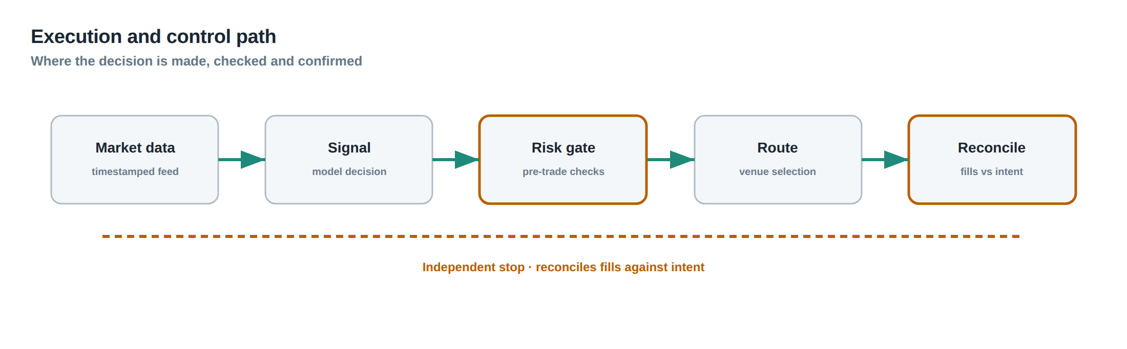
A robust control suite intervenes early in the chain to prevent costly mis‑routing. The first line of defence is a pre‑trade filter that validates the market snapshot against a set of thresholds – for example, rejecting a venue if the queue depth exceeds a multiple of the order size or if the spread exceeds a predefined tolerance.

A second control monitors latency in real time. If the measured one‑way latency for a given path drifts beyond a configurable band, the routing engine automatically switches to an alternative path, even if the decision price is marginally worse. This dynamic latency‑aware routing reduces the probability of arriving at a stale price.

A third safeguard is the “partial‑fill guard”. When an order receives a fill that is smaller than a defined percentage of the requested size within a short time window, the system flags the venue as potentially illiquid and either reduces the remaining quantity or re‑routes the balance to a deeper market.

Finally, a cancellation‑timing rule ensures that cancel requests are sent as soon as the queue depth or adverse‑selection risk breaches a risk‑budget threshold. The rule also caps the maximum time an order may remain alive without a fill, forcing a forced cancel before the order becomes a source of market impact.

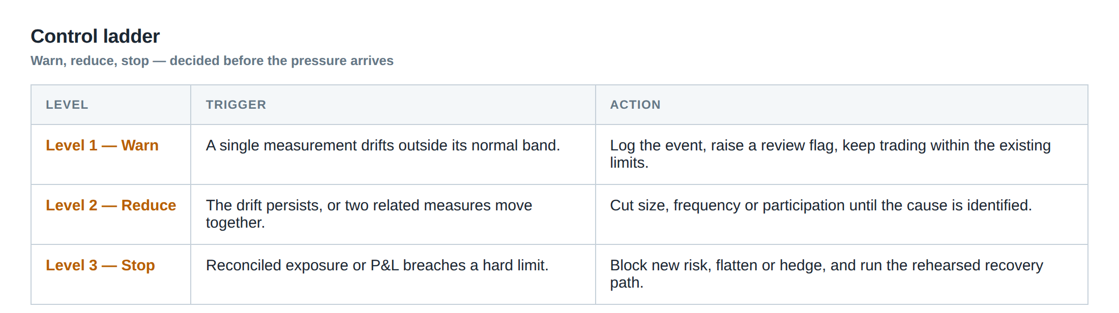
These controls are visualised as a ladder of decision points, each adding a layer of protection before the order reaches the exchange floor.

How to measure whether it is working

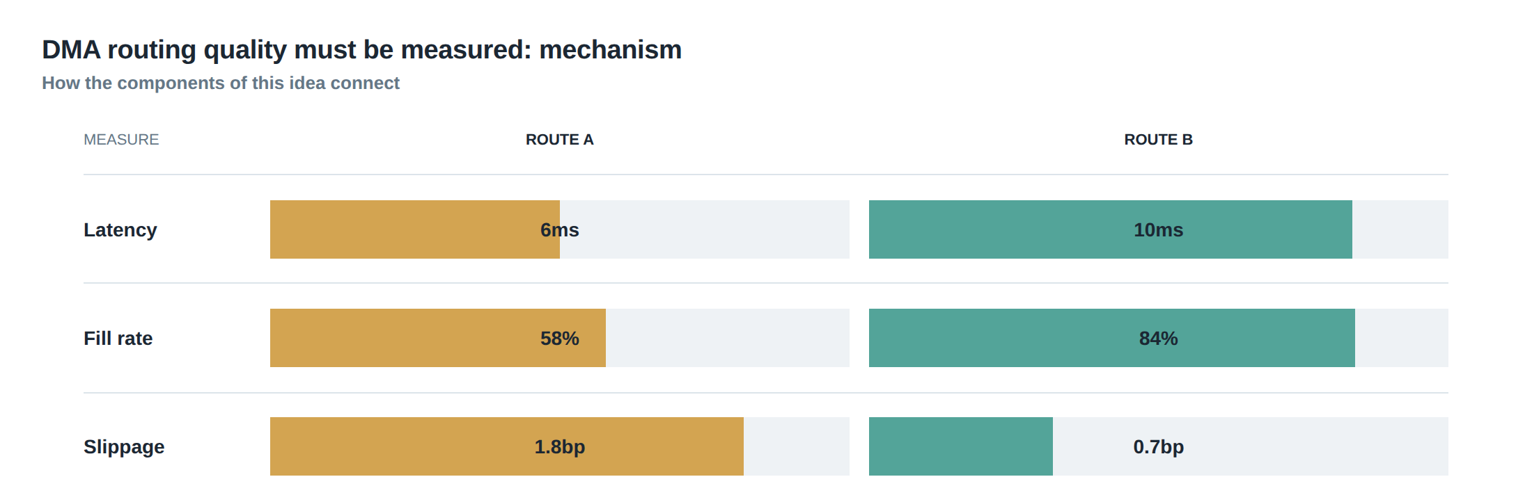
Measurement must be quantitative, repeatable and tied to the same benchmark across venues. The primary metric is the execution slippage, defined as the difference between the final fill price and the decision price, expressed in basis points. A secondary metric is the fill‑rate, the proportion of the original quantity that is executed before cancellation.

Time‑to‑completion is broken into two components: latency‑to‑arrival (network travel time) and queue‑time (time spent waiting for execution). By plotting the distribution of queue‑time against the observed queue depth at arrival, one can infer the marginal cost of each additional share ahead in the line.

Partial‑fill quality is measured by the average price of each partial execution relative to the arrival price, and by the proportion of the order that is filled at each price level. A high proportion of fills at the arrival price indicates that the queue depth estimate was accurate; a drift towards worse prices signals hidden liquidity or adverse selection.

Cancellation outcome is assessed by the “cancellation loss”, i.e. the opportunity cost of the remaining quantity that could have been filled elsewhere at a better price. This is calculated by comparing the market price at the moment of cancel with the price that would have been obtained on the next best venue.

All these metrics are aggregated over a rolling window (e.g., the last 10 000 orders) to smooth out stochastic fluctuations. Statistical significance is tested by comparing the observed slippage distribution against a control sample where orders are routed randomly, ensuring that any improvement is attributable to the routing logic rather than market noise.

The portfolio view

From the desk’s perspective, the quality of DMA routing is not an isolated statistic but a contributor to the overall portfolio performance. Execution slippage directly reduces the realised alpha of each strategy; repeated adverse‑selection costs can erode the edge that the model relies on.

When the routing engine consistently chooses venues that minimise queue‑time, the portfolio benefits from tighter realised spreads, lower inventory holding periods and reduced capital utilisation. Conversely, a systematic bias towards the lowest displayed price without regard to queue depth can inflate the turnover of the portfolio, increase transaction‑cost estimates, and ultimately diminish the Sharpe ratio.

Integrating the routing‑quality metrics into the portfolio‑level risk‑budget allows the desk to allocate execution resources where they generate the highest marginal benefit. For example, a high‑frequency market‑making strategy may tolerate a small increase in latency if it gains a more favourable queue position, whereas a directional macro‑strategy may prioritise the absolute price improvement even at the cost of a longer queue.

By monitoring the aggregate impact of routing decisions on realised P&L, the desk can close the feedback loop: poor execution performance triggers a review of the routing parameters, which in turn refines the decision‑price model and the queue‑depth thresholds. Over time this creates a self‑correcting system that aligns the micro‑level routing choices with the macro‑level portfolio objectives.

In summary, measuring DMA routing quality demands a disciplined approach that captures the full lifecycle of each child order, from decision price through network path, queue interaction, partial fills and cancellation outcomes. Only by quantifying each of these elements can a prop‑trading desk ensure that a direct connection truly adds value rather than merely offering the illusion of speed.

What aspect of your current routing analytics would benefit most from a deeper, queue‑aware measurement framework?

About the research behind this lesson

The seminar frames electronic markets as price-time-priority queues. It separates queue value into spread capture versus adverse-selection cost and the option value of retaining a place in line.

Applied to this lesson: An order lifetime therefore cannot be based on elapsed time alone: the system must reassess whether its queue position, expected spread and adverse-selection risk still justify keeping the order alive.

Explore PULSE: System details

PULSE live account: Verify the live account on FX Blue

Live chat and updates: Telegram @xtrskhft

Source: High-Frequency Trading and Modern Market Microstructure

Educational content only. Trading leveraged products involves risk.