October 14, 2026

What this problem really is

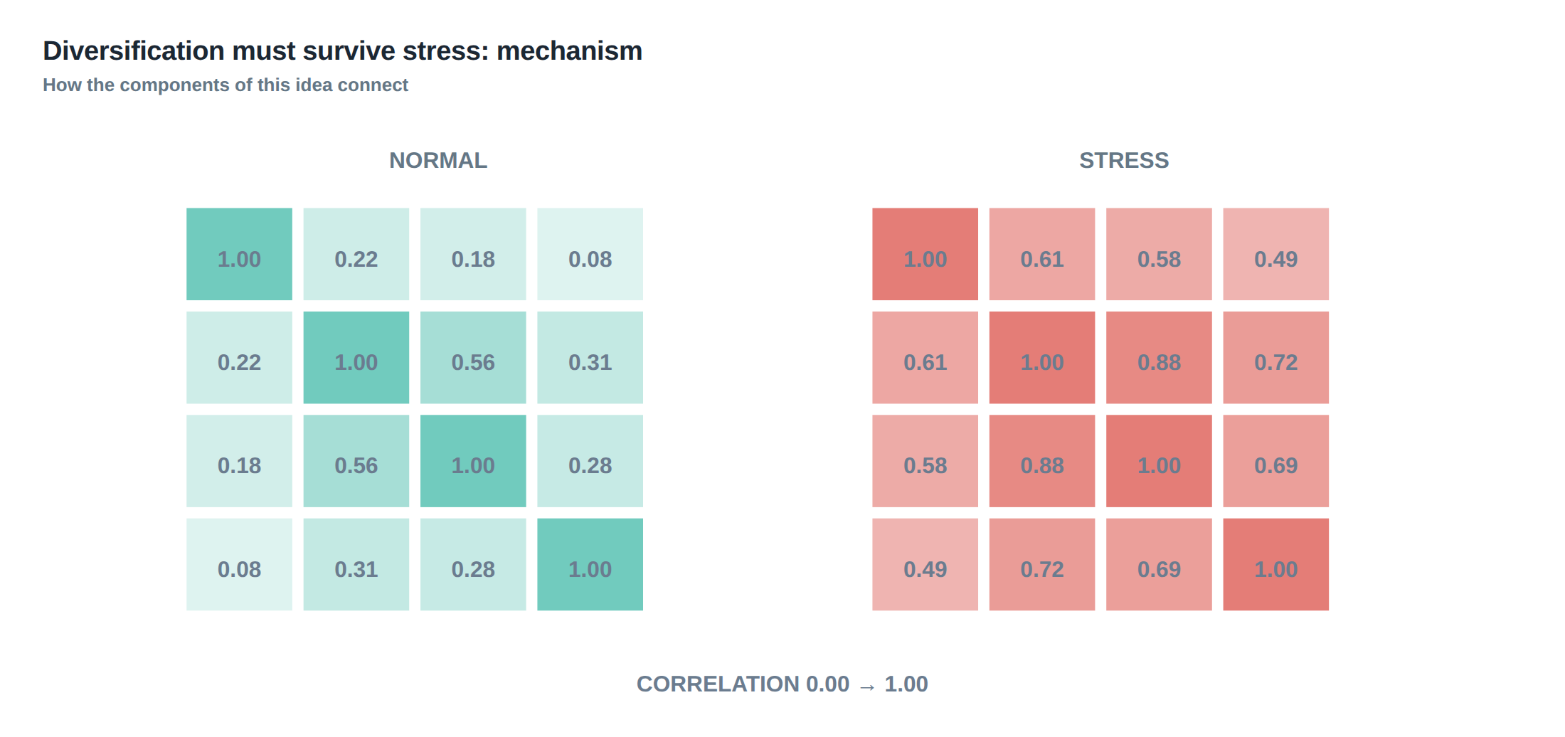
Diversification is traditionally measured on the basis of historic return co‑movements. In calm markets the correlation matrix of a set of strategies often shows modest off‑diagonal values, leading risk managers to conclude that the portfolio will survive a single strategy’s draw‑down. The flaw is that the matrix itself is a snapshot of normal liquidity, funding and volatility conditions. When the market moves from a low‑volatility regime to a stress regime, the same statistical relationships can invert, and the apparent diversification evaporates. The core difficulty, therefore, is not the existence of low average correlation but the fragility of that correlation under the very conditions that trigger risk limits – a sudden spike in funding costs, a rapid widening of bid‑ask spreads, or a cascade of margin calls that forces many participants to liquidate simultaneously.

If the risk framework only monitors average correlation, it will miss the hidden exposure that emerges when a factor shock – for example, a 30 % jump in VIX – pushes spreads on the underlying instruments to their widest levels in years. The same shock also compresses the order book, causing the effective correlation of execution risk to approach one. In that moment the portfolio behaves as a single, highly concentrated position, and any pre‑set limit that assumes diversification will be breached before the monitoring system can react.

The practical implication is that diversification must be stress‑tested as a dynamic property, not a static statistic. The portfolio construction process must embed a “stress‑survival” test that asks whether the correlation structure, liquidity profile and margin utilisation survive a plausible extreme scenario. Only then can the desk set limits that remain meaningful when the market is most unforgiving.

How the mechanism works, step by step

The first step is to build a baseline correlation matrix from a rolling window of returns that is long enough to capture the typical cycle of the strategies, but short enough to remain responsive to regime shifts. Next, a set of factor shocks is defined – for instance, a 200‑basis‑point increase in overnight funding rates, a 50 % widening of the average spread on the most liquid futures, and a 2‑standard‑deviation jump in realised volatility for the equity index.

Each factor shock is then applied to the market microstructure model that drives execution quality. The model translates higher funding costs into larger margin requirements, which in turn reduces the amount of capital each strategy can deploy. Wider spreads raise the cost of entering and exiting positions, while higher volatility expands the realised variance of the price process. By re‑simulating the strategies under these altered conditions, a new correlation matrix is generated that reflects the joint behaviour of the strategies when the market is stressed.

A final step is to compare the stressed matrix to the baseline. If the average off‑diagonal correlation rises by more than a pre‑defined threshold – for example, from 0.12 to 0.45 – the diversification benefit is deemed to have collapsed. At that point the desk must either reduce the aggregate exposure, tighten the concentration limits, or introduce additional hedges that are orthogonal to the stressed factors. The entire pipeline is run on a daily basis, ensuring that the limits are always calibrated to the most recent stress‑adjusted correlation structure.

A worked example with real numbers

Consider two high‑frequency statistical arbitrage strategies, Alpha‑1 and Alpha‑2, that operate on US equity futures. Alpha‑1 generates a daily Sharpe of 1.2, trades an average notional of $10 million per day and holds a margin buffer of 5 % of its gross exposure. Alpha‑2 posts a daily Sharpe of 1.0, trades $8 million per day and maintains a 4 % margin buffer. Over the past twelve months their realised correlation has been 0.14, which would ordinarily be taken as evidence of diversification.

A stress scenario is constructed in which the overnight funding rate jumps by 30 bps, the average bid‑ask spread on the underlying futures widens from 0.5 ticks to 2 ticks, and realised volatility on the S&P 500 futures rises from 12 % annualised to 28 % annualised. The funding shock forces margin requirements to increase from 5 % to 12 % for Alpha‑1 and from 4 % to 10 % for Alpha‑2, leaving each strategy with only half of its usual capital to deploy. The spread widening adds $0.15 per contract to the execution cost, and the volatility surge inflates the daily price variance by a factor of 2.5.

When the two strategies are re‑simulated under these conditions, both experience a simultaneous loss of 15 % of their capital in a single trading day, driven by an inability to unwind positions without paying the widened spread and by forced liquidations triggered by margin calls. The stressed correlation matrix now shows an off‑diagonal value of 0.78, indicating near‑perfect co‑movement. The liquidity‑adjusted concentration metric, defined as the sum of each strategy’s exposure divided by the market’s available depth, jumps from 0.22 in the baseline to 0.61 in stress, well above the desk’s limit of 0.35.

The example demonstrates that low average correlation does not guarantee survivability when the shared liquidity and funding environment collapses. The stress‑adjusted numbers force the risk team to either cut the combined notional to $9 million, increase the margin buffers to 18 %, or introduce a third strategy that is deliberately funded in a different currency and trades a non‑correlated asset class.

Where it breaks in live markets

In real‑time trading the first visible symptom of a breakdown in diversification is a rapid convergence of execution metrics across otherwise unrelated strategies. Order‑book depth shrinks, and the latency distribution of fills becomes heavy‑tailed; a handful of orders that would normally be filled within 1 ms now sit stale for 50 ms or more. This latency spike is often accompanied by a sudden rise in the number of rejected or cancelled orders, a direct consequence of shared margin calls that force the clearing house to tighten collateral requirements across the board.

When several desks are forced to unwind similar positions – for example, a cluster of market‑making algorithms that all hedge delta exposure on the same index – the market experiences a “crowded exit”. The price impact of these simultaneous sells is not linear; each additional unit sold adds more to the spread than the previous one, creating a feedback loop that pushes the realised correlation of returns toward one. The feedback is amplified if the funding environment is already strained, because the cost of borrowing to meet margin calls rises, prompting even more aggressive liquidation.

The breakdown is often observed first on the “liquidity‑adjusted concentration” metric, which spikes as the aggregate notional approaches the thinly‑traded depth of the order book. Once that metric breaches a pre‑set threshold, the risk limit that was based on a benign correlation matrix becomes meaningless – the portfolio is effectively a single, highly leveraged position that can be liquidated only at a severe discount.

The operating path, stage by stage

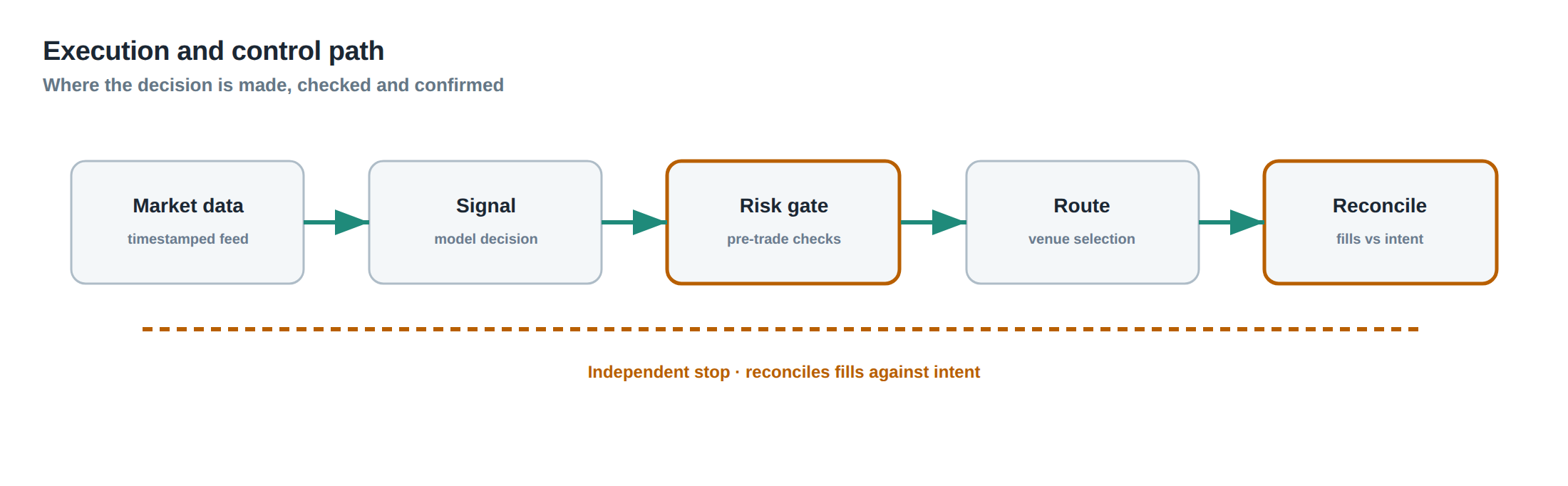
Stage one begins with data ingestion: high‑frequency price, depth, and funding‑rate feeds are normalised and stored in a time‑series database with nanosecond precision. Stage two is the construction of the baseline statistical model, which estimates the mean‑variance‑covariance matrix of strategy returns over the previous 60‑day window and calculates the liquidity‑adjusted concentration for each strategy using the average daily depth of the instruments they trade.

Stage three involves the stress‑generation engine. It draws from a library of calibrated factor shocks – funding spikes, spread widenings, volatility jumps – and applies them to a market‑microstructure simulator that reproduces order‑book dynamics. The simulator outputs a set of synthetic returns for each strategy under each shock scenario.

Stage four aggregates the synthetic returns to produce a stressed correlation matrix and a stressed concentration metric. The system then compares these to the pre‑defined limits: a maximum tolerated correlation increase of 0.30, a concentration ceiling of 0.35, and a margin‑buffer floor of 15 %. If any limit is breached, an alert is raised and the execution engine receives a “diversification‑survival” flag that forces it to throttle order flow, raise spreads, or route to alternative venues.

Stage five is the feedback loop. The risk dashboard records the alert, the mitigation actions taken, and the resulting impact on realised P&L. This information feeds back into the calibration of the factor‑shock library, ensuring that the stress scenarios evolve with market conditions. The whole pipeline runs on a rolling 15‑minute cycle, providing near‑real‑time assurance that diversification remains intact.

Controls that act before the damage

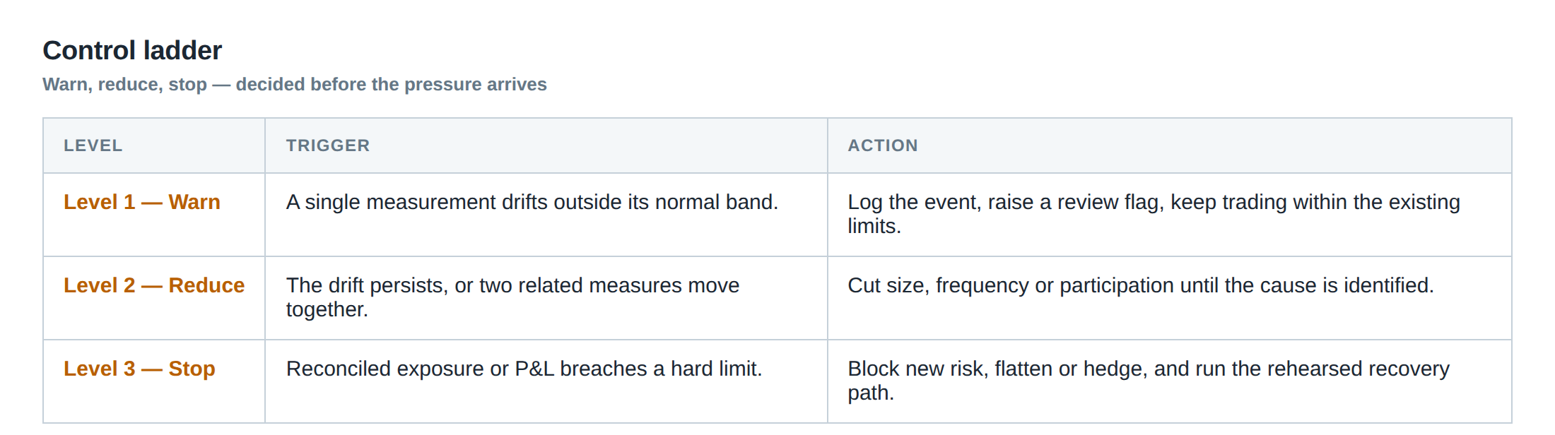
The first line of defence is the pre‑trade liquidity filter, which checks the current market depth against each strategy’s intended notional and refuses to submit orders that would exceed a 20 % utilisation of the available depth. A second control is the dynamic margin‑buffer calculator, which raises the required buffer in proportion to the realised volatility and the observed spread widening; this ensures that the capital cushion expands before a margin call can be triggered.

A third safeguard is the “crowded‑exit detector”. It monitors the aggregate net‑flow of orders across all strategies that share a common underlying and flags when the net sell pressure exceeds the 5 % of daily volume threshold. When the detector activates, the order‑routing logic automatically diversifies execution across less‑correlated venues or spreads the exit over a longer time horizon, reducing the impact on the market price.

The final control is the liquidity‑adjusted concentration monitor, which recalculates the concentration metric in real time using the latest depth data. If the metric approaches the 0.35 limit, the system imposes a hard cap on additional notional for the affected strategies until the metric retreats. These controls are layered so that a failure at any single point does not immediately translate into a portfolio‑wide loss; instead, each layer buys time for the next to engage.

How to measure whether it is working

Effectiveness is measured by comparing the realised co‑movement of strategy returns during periods of market stress to the stressed correlation forecasts generated by the simulation engine. A key performance indicator is the “stress‑adjusted correlation error”, defined as the absolute difference between the forecasted stressed correlation and the realised correlation over the same interval. Consistently low error – for example, below 0.05 – indicates that the stress model captures the true dynamics.

Another metric is the “margin‑call avoidance rate”. This is the proportion of days on which the dynamic margin‑buffer calculator successfully kept the required buffer above the clearing‑house minimum, thereby preventing forced liquidation. A rate above 95 % over a rolling 30‑day window is considered acceptable.

Finally, the “liquidity‑concentration breach frequency” tracks how often the real‑time concentration monitor exceeds its limit. The target is zero breaches; any breach triggers a post‑mortem analysis of the underlying market conditions and a recalibration of the factor‑shock library. By monitoring these quantitative signals, the desk can confirm that the pre‑emptive controls are indeed preserving diversification when it matters most.

The portfolio view

From a portfolio perspective, the central insight is that diversification is a conditional property: it holds only while the market environment satisfies the assumptions embedded in the baseline correlation matrix. By embedding stressed correlation matrices, factor shocks, and liquidity‑adjusted concentration metrics into the risk framework, the desk transforms diversification from a static number into a dynamic safeguard.

The portfolio construction process therefore begins with a “survival test”: each candidate strategy is evaluated not only on its expected return and baseline risk, but also on its contribution to the stressed correlation matrix and its sensitivity to liquidity shocks. Strategies that are highly profitable yet highly sensitive to a common liquidity factor are either down‑scaled or paired with offsetting strategies that thrive when liquidity contracts, such as macro‑fundamental positions that hold cash or low‑beta instruments.

In practice, the portfolio is rebalanced on a weekly cadence, but the stress‑adjusted limits are enforced continuously. When the stressed correlation matrix signals that diversification is eroding, the desk can pre‑emptively trim exposure, raise margin buffers, or introduce new hedges before the market actually forces a convergence of losses. The result is a portfolio that retains its intended risk‑return profile even when the market moves from calm to crisis.

Do you currently test whether the correlation structure of your strategies survives the same stress scenarios that would trigger your margin limits?

About the research behind this lesson

Andrew Lo's lectures build risk analysis from return distributions and statistical measures, rather than treating one realised result as a complete description of risk.

Applied to this lesson: For a fast strategy, median latency or average fill quality is not enough. The review has to include tail delays, stale-order frequency and the loss distribution when cancellation or routing behaves abnormally.

Explore PULSE: System details

PULSE live account: Verify the live account on FX Blue

Live chat and updates: Telegram @xtrskhft

Source: Risk and Return

Educational content only. Trading leveraged products involves risk.