October 6, 2026

What this problem really is

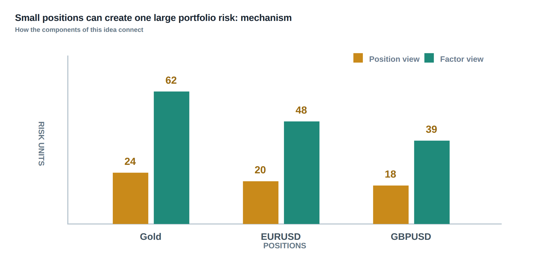
A trader who watches the individual limits on each book often feels comfortable – every position sits well within its prescribed delta, beta, currency and duration caps. The comfort is illusory because the limits are defined in isolation. What is missed is the web of common drivers that bind seemingly unrelated trades together. When a single macro factor – for example a move in the US dollar, a shift in risk‑on sentiment, or a tightening of repo funding – moves, all the “small” positions that share exposure to that factor move in lock‑step. The result is an aggregate exposure that can be many times larger than any single limit would suggest, and which can be amplified under stress when correlations spike. In practice the portfolio behaves as if a single leveraged trade had been entered, even though each leg was modest. The danger is not a one‑off loss but a structural concentration that survives the usual risk‑monitoring screens.

The problem is compounded by the fact that most desks measure exposure on a gross‑not‑net basis, ignoring the offsetting effect of opposite signs that may evaporate when a factor moves. Gross exposure therefore masks the true amount of capital that would be required to unwind the whole book under a severe market move. In a calm market the correlation matrix looks benign; in a crisis it can approach unity, turning a diversified set of bets into a single, massive directional gamble.

How the mechanism works, step by step

First, each strategy is decomposed into a set of factor sensitivities – delta to the underlying price, beta to a market index, currency exposure, duration to interest‑rate shifts, and a volatility‑factor loading. These sensitivities are recorded in a factor‑exposure matrix that is updated in real time. Second, the matrix is multiplied by a correlation matrix that captures how the underlying factors move together. In a tranquil regime the off‑diagonal elements are modest; during a liquidity squeeze they rise sharply. Third, the product yields an aggregate exposure vector that tells the desk how much of each macro driver the whole portfolio actually carries.

When the aggregate exposure exceeds a pre‑defined “stress‑budget”, the system flags a concentration breach even though no single position has breached its own limit. The breach triggers a series of automated checks: are the positions funded through the same repo line? Do they rely on the same order‑book depth? Are they all executed on the same venue where latency spikes are observed? If the answer to any of these is yes, the concentration is considered “liquidity‑linked” and must be reduced or hedged.

Finally, the desk runs scenario‑based stress tests that replace the calm‑period correlation matrix with a stressed version – for example, a 0.9 correlation between the dollar and the risk‑on factor. The resulting aggregate exposures are compared with the capital‑at‑risk limits. If the stressed exposure is larger than the allowed cushion, the desk must either shrink the offending legs or introduce orthogonal hedges that break the common factor link.

A worked example with real numbers

Consider a prop desk that runs five modest long equity‑index futures, each with a notional of USD 2 million. The individual limits are set at a delta of 0.4, a beta of 1.0 to the S&P 500, a currency exposure of zero (all trades are USD‑denominated), a duration of 0 (futures have no carry), and a volatility‑factor loading of 0.2.

The raw sensitivities are therefore:

Position 1: delta 0.4, beta 1.0, vol‑factor 0.2 Position 2: delta 0.35, beta 0.9, vol‑factor 0.18 Position 3: delta 0.38, beta 1.1, vol‑factor 0.22 Position 4: delta 0.42, beta 1.0, vol‑factor 0.19 * Position 5: delta 0.36, beta 0.95, vol‑factor 0.21

In a calm market the correlation between the dollar and the risk‑on factor (the driver of the vol‑factor loading) is estimated at 0.3, and the correlation among the five index futures themselves is 0.5. Multiplying the exposure matrix by this correlation matrix yields an aggregate delta of 1.91, an aggregate beta of 4.85, and a combined volatility‑factor exposure of 1.00.

Now stress the correlations to reflect a “risk‑on” episode: the dollar‑risk‑on correlation jumps to 0.85 and the inter‑future correlation rises to 0.9. Re‑computing gives an aggregate delta of 3.57, an aggregate beta of 9.12, and a volatility‑factor exposure of 1.86. In effect, the five modest trades now behave like a single leveraged position with a delta close to 4 × the original per‑trade limit and a beta more than nine times a single‑trade cap.

If the desk’s capital‑at‑risk budget for beta is 6, the stressed beta of 9.12 breaches the limit by 52 %. The gross exposure (sum of absolute betas) is 5.0, the net exposure (sum with signs) is also 5.0 because all trades are long, but the stressed exposure is 9.12, illustrating how stress‑testing can reveal hidden concentration that gross and net numbers hide.

The example also shows a financing dependency: all five futures are margined through the same overnight repo line that sources funding at a rate linked to the USD‑LIBOR curve. A sudden spike in repo rates would increase funding costs across the board, creating a second‑order liquidity shock that compounds the market move.

Where it breaks in live markets

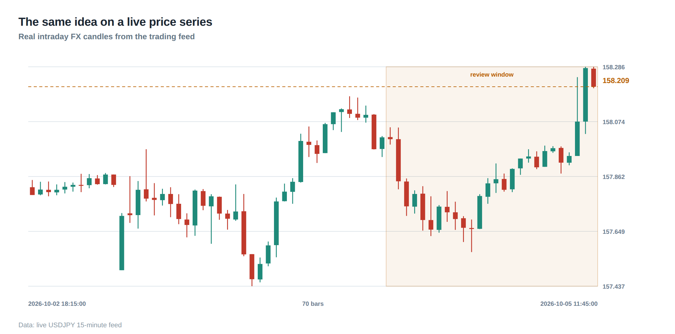
In live trading the assumptions that keep the correlation matrix tame are constantly violated. Market microstructure noise, order‑flow clustering, and the rapid unwinding of correlated positions by other market participants can push correlations to near unity within minutes. When a major macro announcement – for example a surprise change in the Federal Reserve policy – hits, the dollar often moves in tandem with risk‑on equities, and the volatility surface re‑prices across asset classes.

Execution venues also add fragility. If the five futures are all routed to the same exchange, a temporary order‑book freeze or a latency spike can cause a cascade of stale orders. The latency distribution, which is usually summarised by a median of 2 ms, develops a heavy tail: a 5 % tail of 30 ms or more. Those tail events are precisely the moments when the portfolio’s aggregate exposure is most vulnerable, because the market may have already moved on the common factor while the desk is still attempting to fill stale orders.

Funding markets are another breaking point. During a repo squeeze, the overnight funding rate can double, and the cost of maintaining the margin on all five futures rises simultaneously. The desk’s financing model, which normally assumes a stable cost of capital, is forced into a stress scenario that it has not explicitly priced. The combination of market‑price moves, execution delays, and funding cost spikes creates a perfect storm where the “small” positions collectively generate a loss comparable to a large, highly leveraged position.

The operating path, stage by stage

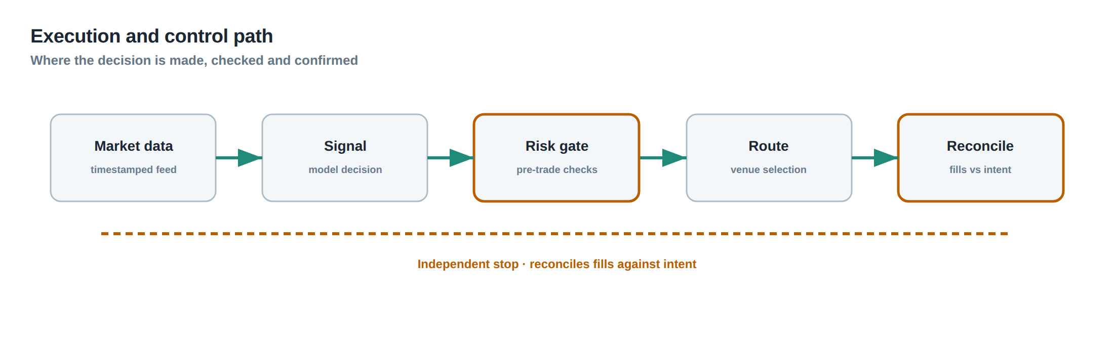
The first stage is data ingestion: market data, order‑book snapshots, and funding rates are streamed into a central risk engine. The engine normalises the data, calculates real‑time factor sensitivities for each position, and stores them in a high‑frequency exposure table.

The second stage is correlation estimation. A rolling window of 30 minutes is used to compute the covariance matrix of the underlying factors. The window is deliberately short to capture rapid regime shifts, but a secondary “stress‑window” of the last 24 hours is also maintained to provide a baseline for stressed correlation levels.

The third stage is aggregation. The exposure table is multiplied by the current correlation matrix to produce the aggregate exposure vector. Simultaneously, the same multiplication is performed with the stress‑window matrix, yielding a stressed‑exposure vector.

The fourth stage is limit checking. Both the live and stressed vectors are compared against a hierarchy of limits: per‑trade, per‑strategy, and portfolio‑wide. Breaches trigger alerts that are routed to the desk’s risk manager and, if the breach is severe, to an automated position‑reduction engine.

The fifth stage is response. The desk may execute a hedge that is orthogonal to the offending factor – for example, a short USD‑JPY forward to reduce dollar exposure – or it may unwind the most correlated legs. The response is logged, and the outcome feeds back into the data ingestion stage, closing the loop.

Controls that act before the damage

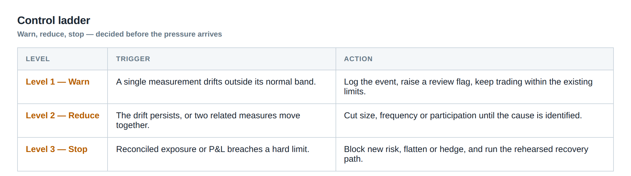
Preventive controls begin with the construction of the factor‑exposure matrix. By insisting that every new strategy submit a complete list of factor loadings, the desk ensures that hidden commonalities are visible from the outset. A second control is the “liquidity ladder”: each strategy is assigned a tier based on the depth of the market it trades, the funding source it uses, and the latency profile of its order routing. Strategies that sit on the same rung of the ladder are prohibited from holding more than a pre‑set aggregate exposure to any single factor.

A third control is the pre‑trade stress test. Before a trade is approved, the engine runs a hypothetical scenario where all relevant correlations are set to their stressed values. If the resulting aggregate exposure would breach a limit, the trade is rejected or required to be re‑sized.

A fourth control is the funding‑capacity buffer. The desk maintains a reserve of high‑quality liquid assets that can be deployed to meet sudden margin calls without resorting to the same repo line that finances the majority of the portfolio. This buffer reduces the coupling between market moves and financing costs.

Finally, the desk enforces a “latency‑tail” monitoring rule. Instead of only tracking median fill times, the system records the 95th‑percentile latency and raises an alert if it exceeds a threshold that would materially affect the execution of correlated trades. By catching latency tail events early, the desk can pause new order flow and re‑balance the portfolio before a cascade develops.

How to measure whether it is working

Effectiveness is gauged by comparing the realised aggregate exposure against the theoretical exposure predicted by the risk engine. A key metric is the “exposure tracking error”, defined as the standard deviation of the difference between realised and modelled aggregate delta over a rolling window. A low tracking error indicates that the factor model is capturing the true dynamics of the portfolio.

Another metric is the “stress‑breach frequency”. This counts how often the stressed‑exposure vector exceeds its limit in a given month. A decreasing frequency over time suggests that the preventive controls are successfully limiting concentration.

Capital utilisation is also examined. The ratio of capital allocated to the “liquidity ladder” buffer versus the total capital at risk should remain within a target band (for example 5‑10 %). If the buffer is consistently under‑utilised, the desk may be over‑conservative; if it is frequently depleted, the controls are insufficient.

Lastly, the desk tracks the tail of the latency distribution. The 99th‑percentile latency should stay below a pre‑agreed threshold (e.g., 40 ms). Any breach triggers a post‑mortem analysis to determine whether the latency spike coincided with an increase in aggregate exposure, thereby confirming the link between execution risk and factor concentration.

The portfolio view

From a portfolio perspective the most reliable picture is obtained by looking at exposure in three dimensions: gross, net and stressed. Gross exposure aggregates the absolute values of each factor loading, ignoring sign. Net exposure sums the signed loadings, showing the directional tilt. Stressed exposure applies a stress‑correlation matrix to the factor loadings, revealing the hidden concentration that would emerge under market duress.

A well‑balanced portfolio will have gross exposure that is comfortably below the capital limit, net exposure that is close to zero for the most volatile factors, and stressed exposure that remains within a modest margin of the stress‑budget. When any of these three diverge – for example, when stressed beta spikes while gross and net remain tame – the desk knows that a hidden concentration has formed.

The portfolio view also incorporates financing and liquidity dimensions. By overlaying the exposure map with the funding sources and venue‑usage heat‑map, the desk can spot clusters where many positions depend on the same repo line or the same exchange. Those clusters are candidates for diversification, either by moving a subset of trades to a different venue or by sourcing funding from a separate counterparty.

In practice the portfolio view is displayed on a live dashboard that refreshes every second, showing colour‑coded bars for gross, net and stressed exposure across delta, beta, currency, duration and volatility‑factor axes. The dashboard also flags any ladder‑tier breaches and latency‑tail alerts, giving the trader a single pane of glass that summarises the multidimensional risk that would otherwise be hidden behind individual limits.

Do you currently monitor the stressed‑correlation exposure of your modest positions, or do you rely solely on per‑trade limits to keep your portfolio safe?

About the research behind this lesson

Andrew Lo's lectures build risk analysis from return distributions and statistical measures, rather than treating one realised result as a complete description of risk.

Applied to this lesson: For a fast strategy, median latency or average fill quality is not enough. The review has to include tail delays, stale-order frequency and the loss distribution when cancellation or routing behaves abnormally.

Explore PULSE: System details

PULSE live account: Verify the live account on FX Blue

Live chat and updates: Telegram @xtrskhft

Source: Risk and Return

Educational content only. Trading leveraged products involves risk.