October 6, 2026

What this problem really is

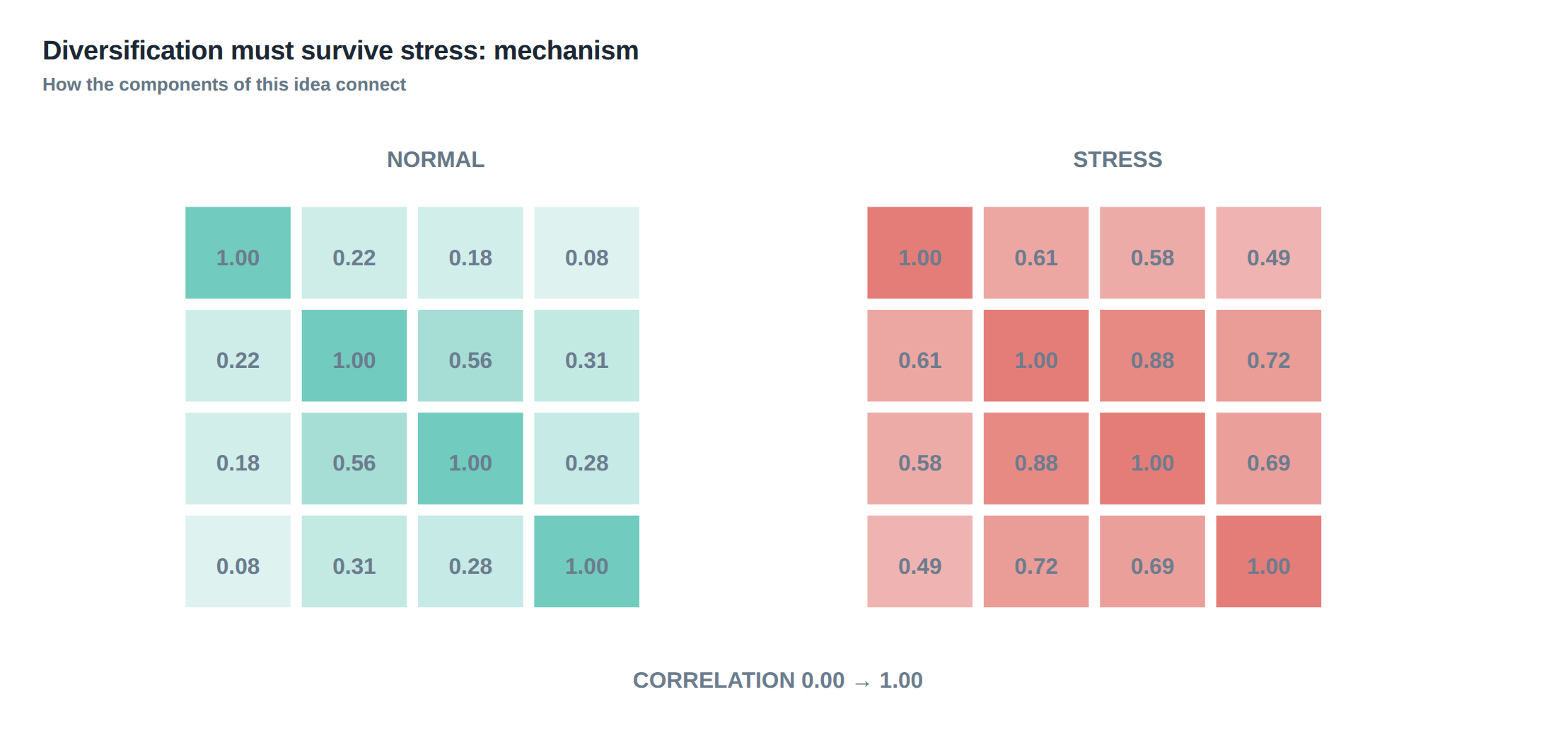
Diversification is traditionally measured on the basis of historic return correlations observed during tranquil market periods. The assumption that a low average correlation guarantees that losses will be spread out collapses when the market moves from a regime of ample liquidity to one of stress. In a stressed environment the statistical relationships that underpin portfolio construction are themselves subject to rapid change; assets that have behaved independently can become tightly coupled through common funding constraints, margin calls, and the simultaneous widening of bid‑ask spreads. The practical consequence for a prop‑trading desk is that a portfolio that appears well‑balanced on a static correlation matrix may, in the seconds before a limit breach, behave as a single, highly concentrated exposure.

The core difficulty is that risk limits are most likely to be tested precisely when the correlation structure that justified those limits is no longer valid. A strategy that normally trades on a tight spread may see that spread double while volatility spikes, and the same liquidity shock that forces a short‑term squeeze on one instrument may trigger a cascade of margin calls across unrelated desks. The resulting “correlation breakdown” is not a statistical artefact but a structural shift driven by shared balance‑sheet pressures.

Because the breakdown is regime‑dependent, a portfolio that survives a 20‑percent draw‑down in a calm market can be wiped out by a 5‑percent move when liquidity evaporates. The problem is therefore not a lack of diversification in the conventional sense, but the failure of the diversification framework to survive the stress that activates the very limits it was designed to protect.

How the mechanism works, step by step

The first step is the construction of a stressed correlation matrix. Instead of using the sample covariance of daily returns, the desk builds a matrix that incorporates factor shocks derived from historical crisis episodes – for example, a 30‑basis‑point jump in the 5‑year Treasury yield, a 40‑percent widening of the S&P 500 index spread, and a simultaneous 25‑percent increase in implied volatility across the equity options surface. Each shock is applied to the factor loadings of the individual strategies, producing a new set of implied correlations that reflect the joint impact of market‑wide stressors.

Second, the desk simulates simultaneous spread widening and volatility expansion. A spread‑based market‑making strategy that normally earns a 0.5‑bp rebate on a 1‑bp spread may, under stress, see that spread widen to 5 bp while volatility doubles. The same simulation is run for a statistical‑arbitrage strategy that relies on tight execution latency; the model imposes a tail‑delay distribution that captures the probability of order‑routing failures when network queues lengthen.

Third, the model adds the effect of crowded exits and shared margin calls. When several desks attempt to unwind similar positions, the order flow overwhelms the market, forcing price impact to increase sharply. At the same time, the reduction in collateral value triggers margin calls that are satisfied by liquidating assets across desks, reinforcing the price move. This feedback loop is represented by a coupling term that raises the off‑diagonal elements of the stressed correlation matrix in proportion to the concentration of margin‑call exposure.

Finally, the desk recomputes a liquidity‑adjusted concentration metric. The metric weights each strategy’s notional by the inverse of its average market depth and by a funding stability factor that reflects the proportion of capital that is financed on a short‑term repo basis. The resulting number replaces the naïve notional‑weighted concentration used in normal‑market risk reports, and it is compared against a pre‑set limit that is deliberately tighter than the conventional diversification threshold.

A worked example with real numbers

Consider two strategies: a high‑frequency statistical‑arbitrage (StatArb) desk that trades a basket of US equity futures, and a mid‑frequency spread‑capture (SpreadCap) desk that provides liquidity in the EUR/USD‑GBP/USD cross. Over the past twelve months the daily return correlation between the two has been 0.07, well below the typical 0.2‑0.3 threshold used to deem a pair “diversified”. The StatArb desk holds an average gross exposure of $150 million, with an average market depth of 2,000 contracts and a funding cost of 0.4 % per annum on a 30‑day repo. The SpreadCap desk carries $120 million gross exposure, an average depth of 1,500 contracts, and funds 70 % of its capital on a 10‑day commercial paper line at 0.6 % per annum.

In a normal‑market stress test the desk applies a 20‑basis‑point shock to the 5‑year Treasury curve, a 15‑percent widening of the EUR/USD‑GBP/USD spread, and a 30‑percent increase in the VIX. The stressed correlation matrix rises from 0.07 to 0.42, reflecting the common funding squeeze. Simultaneously the StatArb model imposes a tail‑delay probability of 0.12 that an order will be delayed by more than 200 µs, which historically adds a 1.2‑percent tail loss to the strategy’s P&L distribution. The SpreadCap model shows a spread widening from 3 bp to 12 bp, inflating the expected trading cost by $4.8 million per day.

When the stress scenario is run, the combined daily VaR at the 99.5 % level jumps from $2.3 million (normal) to $7.9 million (stressed). The liquidity‑adjusted concentration metric, defined as Σ (notional × 1/depth × funding‑instability), moves from 0.018 in the calm case to 0.045 under stress, crossing the pre‑agreed limit of 0.04. The desk therefore flags that the diversification that existed in the calm matrix has effectively disappeared, and it must either reduce notional, increase depth, or secure longer‑term funding before the next trading day.

Where it breaks in live markets

The theoretical framework collapses when the assumptions embedded in the stress matrix no longer capture the speed of market deterioration. In a flash‑crash scenario the order‑book depth can evaporate within a handful of milliseconds, a timescale that is invisible to a model that updates liquidity metrics on a five‑minute grid. The same applies to funding shocks; a sudden downgrade of a counterparty can force a repo market to seize up, turning a 30‑day funding cost of 0.4 % into an overnight spike of 2 % and instantly invalidating the funding‑instability factor.

Crowded exits are another point of failure. When several desks receive a margin‑call at the same price level, the aggregate sell pressure can push the price beyond the range assumed by the spread‑widening shock. The model’s linear coupling term underestimates the non‑linear price impact that arises from order‑book depletion, leading to an under‑estimation of the post‑stress correlation.

Finally, the measurement of tail delays in latency‑sensitive strategies often relies on historical distribution tails that are thin because extreme network congestion events are rare. In a real‑time outage, the distribution can shift dramatically, creating a “black‑swan” delay that is not represented in the simulated tail‑delay probability. The result is a sudden loss of execution quality that can turn a modest spread capture into a sizeable slippage loss, eroding the diversification benefit in real time.

The operating path, stage by stage

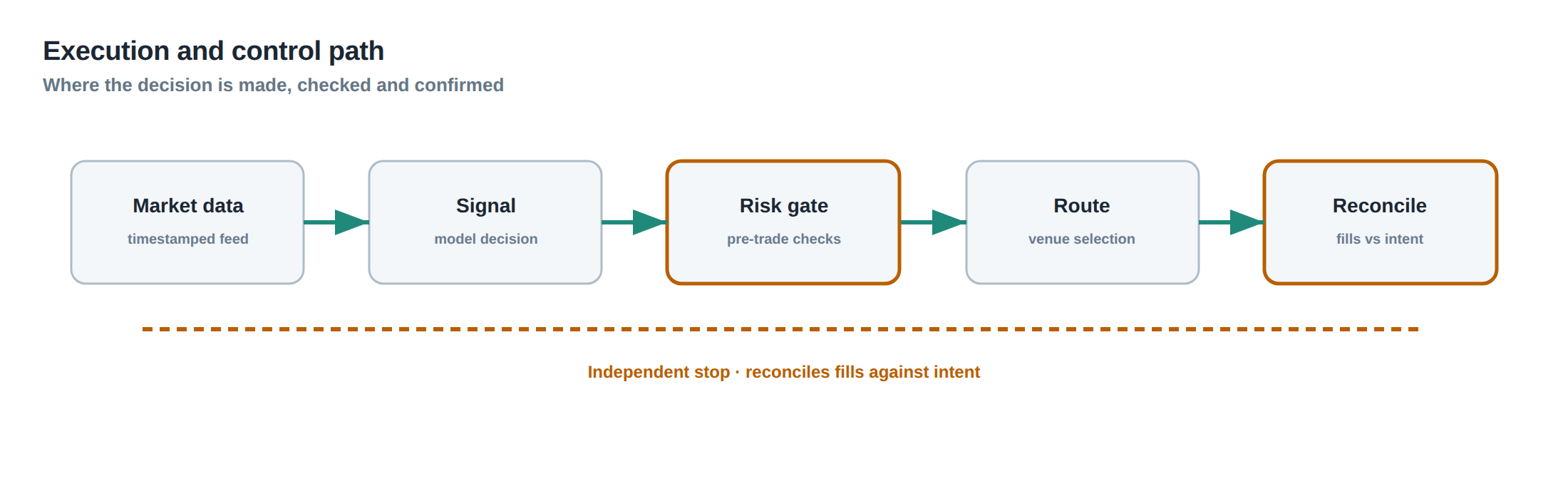
The first stage is data ingestion. The desk continuously records market depth, spread, volatility, and funding rates at sub‑second resolution. These streams are fed into a rolling window that computes factor sensitivities for each strategy, updating the base correlation matrix on a fifteen‑minute cadence.

The second stage is stress generation. A library of historic crisis factor shocks is maintained, each calibrated to a specific market‑wide event such as a sovereign default or a liquidity crunch in the repo market. The library is combined with a Monte‑Carlo engine that draws random combinations of shocks, preserving the observed co‑occurrence frequencies.

The third stage is scenario evaluation. For each drawn shock, the engine recomputes the factor loadings, the stressed correlation matrix, and the liquidity‑adjusted concentration metric. The engine also simulates the simultaneous spread widening and volatility expansion, applying the appropriate cost and tail‑loss adjustments to each strategy’s P&L distribution.

The fourth stage is limit checking. The resulting VaR, stressed concentration, and projected margin‑call exposure are compared against a hierarchy of limits: a primary diversification limit, a secondary liquidity‑adjustment limit, and a tertiary funding‑instability limit. If any limit is breached, the system raises an alert that propagates to the desk manager and the risk operations team.

The final stage is execution control. Upon an alert, the desk automatically scales down the affected strategies, either by reducing order flow, widening quoting bands, or shifting to a longer‑term funding source. The control actions are logged and fed back into the next iteration of the data ingestion stage, ensuring that the system learns from each stress event.

Controls that act before the damage

The first line of defence is a pre‑trade liquidity filter. Before any order is sent, the system checks the current market depth against a minimum threshold derived from the strategy’s average depth and the stressed depth implied by the most recent factor shock. If the depth falls below the threshold, the order is either throttled or cancelled.

A second control is the funding‑stability buffer. The desk maintains a reserve of long‑dated collateral that can be deployed when short‑term repo rates spike. The buffer size is calibrated to the worst‑case funding‑instability factor observed in the stress library, ensuring that a sudden increase in funding cost does not immediately trigger a margin call.

The third control is a dynamic concentration cap. The liquidity‑adjusted concentration metric is recomputed in real time, and the system enforces a hard cap that is lower than the static notional‑weighted cap used in normal markets. When the metric approaches the cap, the system automatically reduces exposure by scaling down order sizes across all strategies that share the same liquidity source.

A fourth safeguard is a “crowded‑exit” detector. The detector monitors the aggregate net change in open interest across all desks that trade the same underlying. If the net change exceeds a pre‑set percentage of the average daily turnover, the detector flags a potential crowded unwind and forces a temporary halt on new position builds for the affected instruments.

These controls are layered so that a failure at one level is compensated by the next, creating a robust barrier that preserves diversification until the market stress subsides.

How to measure whether it is working

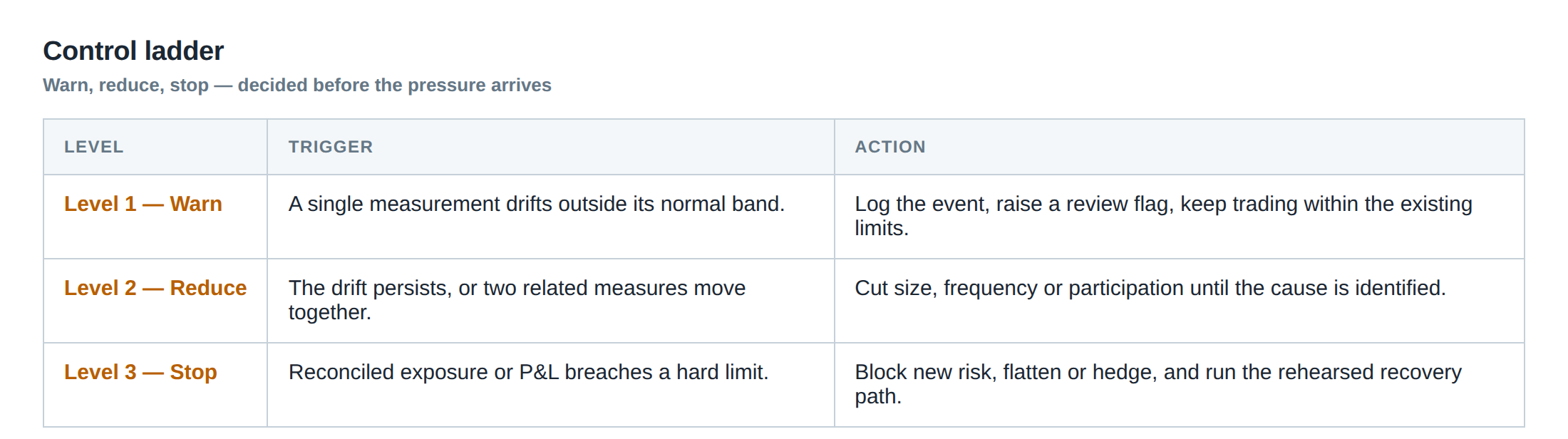
Effectiveness is measured by tracking the realised versus stressed concentration gap. The gap is the difference between the liquidity‑adjusted concentration observed in live trading and the same metric projected by the most recent stress scenario. A narrowing gap over successive weeks indicates that the stress model is capturing the dominant sources of correlation shift.

Another metric is the frequency of limit breaches after the implementation of the dynamic concentration cap. A reduction in breach frequency, combined with a stable or improved Sharpe ratio, suggests that the controls are preventing the loss of diversification without unduly curtailing return.

The third measurement is the tail‑delay capture rate. By logging the actual latency distribution and comparing the observed tail‑delay frequency to the modelled tail‑delay probability, the desk can quantify how well the latency‑risk component is calibrated. A convergence of the two indicates that the latency stress factor is correctly sized.

Finally, the desk monitors the realised funding‑instability cost during periods of market stress. The realised cost is compared to the worst‑case funding shock used in the stress library. If the realised cost consistently remains below the shock, the funding buffer is appropriately sized; if it exceeds the shock, the library must be expanded to include more severe funding events.

The portfolio view

From the portfolio perspective, diversification must be treated as a dynamic state rather than a static label. The portfolio’s risk profile is a function of three interacting dimensions: correlation, liquidity, and funding. Each dimension is regime‑dependent, and the transition between regimes is often triggered by the same market stress that forces a limit breach.

When the stressed correlation matrix shows a rise from 0.07 to 0.42, the portfolio’s effective number of independent bets collapses from roughly ten to three. The liquidity‑adjusted concentration metric then rises, signalling that the remaining independent bets are being funded through a narrower set of market venues. If the funding‑instability factor simultaneously spikes, the portfolio’s margin‑call exposure becomes highly correlated across desks, creating a single point of failure.

The appropriate response is to monitor the three dimensions in concert, to set limits that are tighter than the static thresholds used in calm markets, and to enforce controls that act before the correlation structure collapses. By doing so, a prop‑trading desk can preserve the true benefit of diversification – the ability to absorb shocks without breaching risk limits – even when the market environment is shifting beneath its feet.

Will your current diversification framework survive the next liquidity shock, or will it crumble before you have a chance to act?

About the research behind this lesson

Andrew Lo's lectures build risk analysis from return distributions and statistical measures, rather than treating one realised result as a complete description of risk.

Applied to this lesson: For a fast strategy, median latency or average fill quality is not enough. The review has to include tail delays, stale-order frequency and the loss distribution when cancellation or routing behaves abnormally.

Explore PULSE: System details

PULSE live account: Verify the live account on FX Blue

Live chat and updates: Telegram @xtrskhft

Source: Risk and Return

Educational content only. Trading leveraged products involves risk.