October 7, 2026

What this problem really is

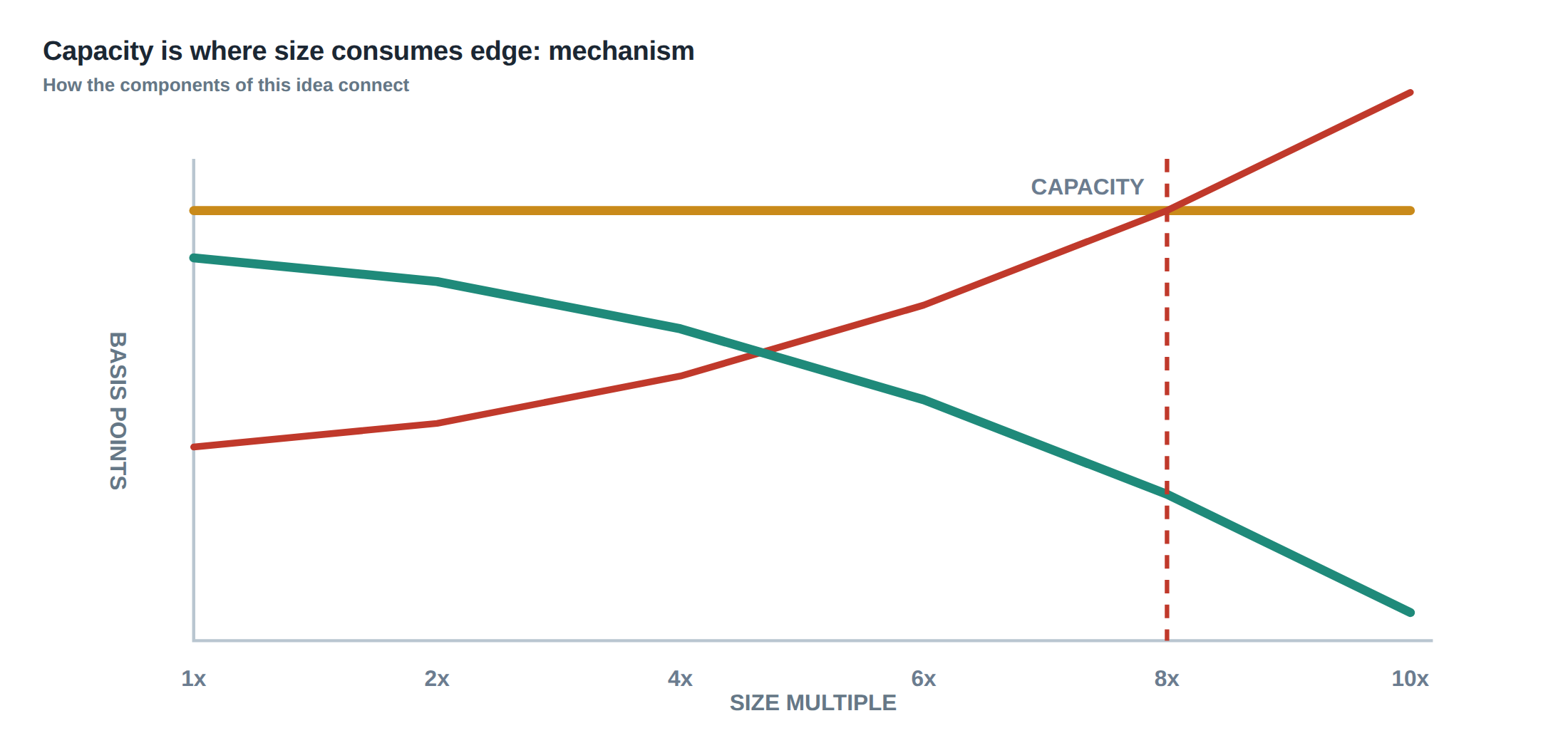
In electronic markets the most visible metric of a strategy’s profitability is the spread it captures. Yet the spread is only a part of the picture; the moment a trader begins to add size, the order itself reshapes the price formation process. When the quantity required to realise the theoretical edge is large enough to push the execution into deeper parts of the limit‑order book, the realised P&L can be eroded or even reversed. This phenomenon is commonly described as “capacity”: the point at which the market’s ability to absorb additional volume without moving price collapses, and the trader’s own orders become the dominant source of cost. The problem is not simply that commissions rise with turnover, but that the market impact, both temporary and permanent, and the opportunity cost of waiting for a favourable queue position rise faster than the nominal edge. Consequently a strategy that appears robust at a few hundred contracts can become unprofitable when the desk attempts to scale to the millions required for a meaningful portfolio contribution.

How the mechanism works, step by step

The first step is to model the four principal cost components that compete against the raw spread: (1) the quoted spread itself, which is the immediate price improvement a limit order can obtain; (2) temporary impact, the short‑lived price concession incurred while the order is being filled; (3) permanent impact, the lasting shift in the mid‑price that remains after the order is completed; and (4) opportunity cost, the expected loss from not being in the queue when a favourable price move occurs. Temporary impact can be expressed as a function of participation rate – the ratio of order flow to total market volume – multiplied by a volatility‑scaled coefficient. Permanent impact is often approximated as a fraction of the temporary impact, reflecting the market’s tendency to incorporate large trades into its price discovery. Opportunity cost is linked to the expected time to execution, which itself depends on the depth of the queue and the volatility of the instrument. By quantifying each component, a trader can construct a “capacity curve” that maps expected net edge against order size.

The second step is to stress‑test the model under adverse market conditions. Thin trading sessions, such as the opening hour of a less‑liquid equity or the after‑hours window of a futures contract, have markedly lower depth and higher volatility. In those windows the participation rate required to achieve a given size spikes, inflating temporary impact dramatically. Similarly, when a position must be unwound urgently – for example after a sudden adverse move – the trader may be forced to cross the spread or accept a worse price than the model predicts. By simulating these scenarios the desk can identify the size at which the expected net edge first reaches zero, which is the practical capacity limit for that strategy.

A worked example with real numbers

Consider a mean‑reversion market‑making model on a highly liquid equity that, on average, captures a 2‑cent spread per share. The model predicts a temporary impact coefficient of 0.5 cents per 10 % participation, and a permanent impact that is 30 % of the temporary impact. The average daily volume (ADV) is 5 million shares, and the realised volatility over a 5‑minute window is 0.8 cents.

A baseline trade of 10 000 shares represents a participation rate of 0.2 % (10 000 / 5 000 000). The temporary impact is therefore 0.5 cents × 0.2 = 0.1 cents, and permanent impact is 0.03 cents. Opportunity cost, estimated as the product of volatility and expected waiting time (≈2 minutes), adds roughly 0.16 cents. Summing costs gives 0.29 cents, leaving a net edge of 1.71 cents per share, or a gross expectancy of $171 on the 10 000‑share trade.

Now double the size to 20 000 shares. Participation rises to 0.4 %, so temporary impact becomes 0.5 cents × 0.4 = 0.2 cents, permanent impact 0.06 cents, and the order must walk down two additional price levels in the book, widening the effective spread to 3 cents. The opportunity cost also grows because the queue position is deeper; the expected waiting time lengthens to about 4 minutes, adding 0.32 cents. Total cost is now 0.58 cents, while the spread capture is only 1.5 cents (2 cents minus the extra 0.5 cent depth). Net edge collapses to 0.92 cents per share, a 46 % reduction in profitability despite a 100 % increase in notional. If the trader were to push the size to 40 000 shares, participation reaches 0.8 %, temporary impact climbs to 0.4 cents, permanent impact 0.12 cents, and the order must consume the entire top of the book, effectively paying the full quoted spread. The net edge becomes negative, illustrating how doubling quantity can more than double cost when the extra order must trade through deeper and worse price levels.

Where it breaks in live markets

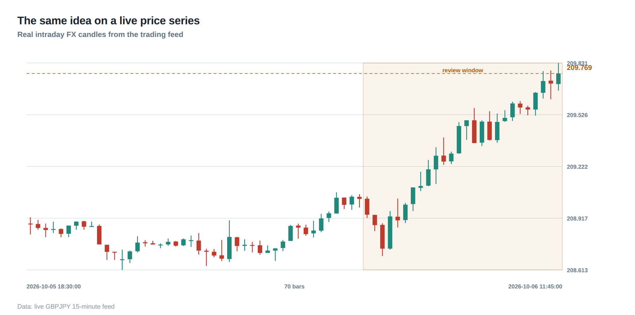
In theory, the capacity curve is smooth and predictable, but live markets inject stochastic shocks that can cause abrupt departures from the model. During a thin session, the order book may contain only a few hundred shares on each side; a modest increase in participation can instantly consume the entire displayed depth, forcing the algorithm to “lift” the offer and pay the full spread plus a slippage component that is not captured by the volatility‑scaled coefficient. Likewise, news releases or macro events can spike volatility, inflating the opportunity‑cost term faster than the model can adjust. Urgent exits exacerbate the problem: a trader who must liquidate a large position within seconds cannot rely on the expected waiting time, and the realised temporary impact may be several times the calibrated value. In such environments the realised P&L curve bends sharply downward, and the strategy’s edge can evaporate in a single bar.

The operating path, stage by stage

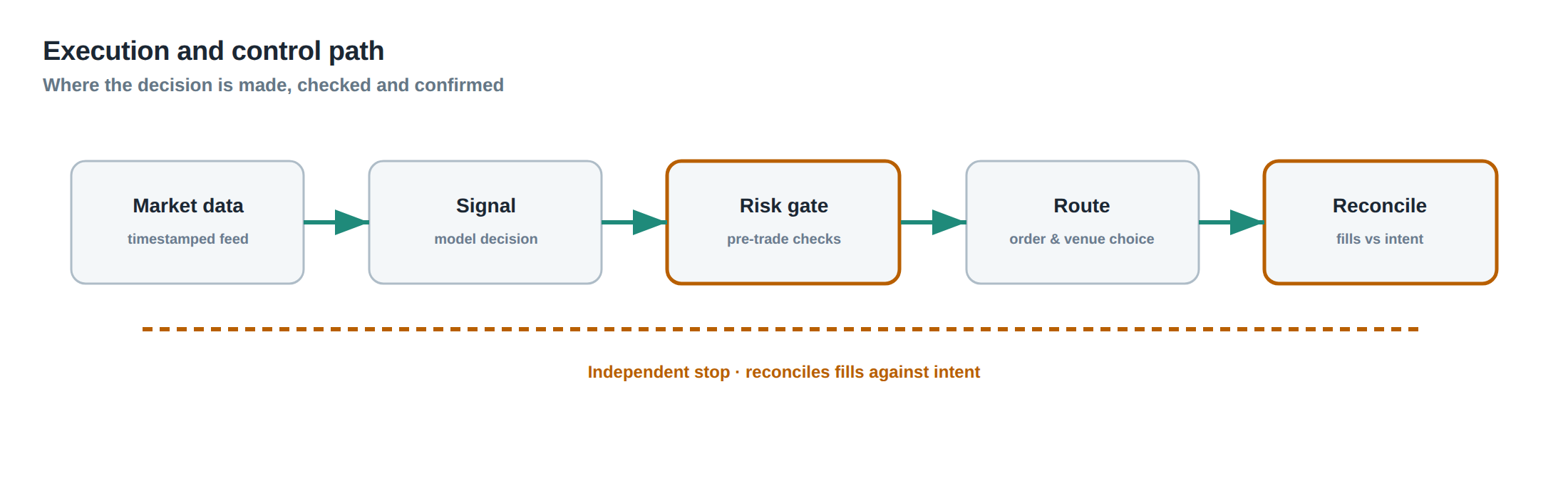
The operational workflow begins with a pre‑trade simulation that incrementally raises order size while recomputing the capacity curve. The simulation stops when the expected net edge falls to zero, and that size is recorded as the “capacity ceiling” for the instrument and time‑slice. In the execution stage, the order management system (OMS) monitors real‑time participation rate, market depth, and realised volatility. If any metric exceeds a predefined threshold – for example, participation above 0.5 % in a 5‑minute window – the OMS throttles the order flow or switches to a more passive posting strategy. Should the order’s queue position deteriorate beyond the point where the expected spread capture no longer outweighs the accrued temporary impact, the system automatically cancels and re‑quotes at a deeper level. Throughout the trade, a “capacity guard” module compares live slippage against the pre‑computed curve; any divergence triggers an alert and may invoke a risk‑off mode that reduces exposure across the portfolio.

Controls that act before the damage

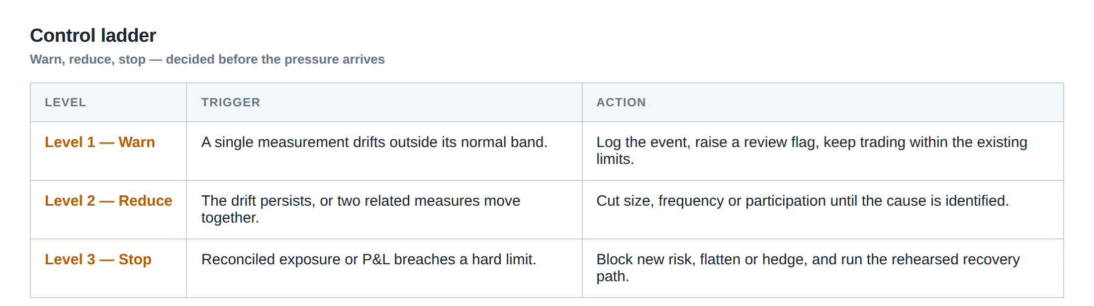
Preventative controls are layered to catch capacity breaches before they translate into realised loss. The first line is a static participation‑rate limit that is calibrated per instrument and session; it caps the maximum flow that any single strategy may inject into the market. The second line is a dynamic depth‑monitor that watches the cumulative volume at the best price levels; when the remaining depth falls below a multiple of the intended order size, the system reduces aggressiveness. A third safeguard is a “queue‑value” estimator that decomposes the expected profit of staying in line into spread capture, adverse‑selection risk, and the option value of retaining position. If the option value turns negative, the algorithm removes the order regardless of elapsed time. Finally, a “stress‑test scheduler” runs overnight simulations that inject synthetic spikes in volatility and drops in depth, updating the capacity ceiling for the next trading day. By embedding these controls into the order‑routing logic, the desk can keep the realised edge comfortably above the theoretical minimum.

How to measure whether it is working

Measurement is an ongoing, data‑driven exercise. The primary metric is the realised net edge per share, calculated as the captured spread minus the sum of temporary impact, permanent impact, and opportunity cost. This figure is plotted against the simulated capacity curve for each instrument; the distance between the two lines indicates model fidelity. A secondary metric is the slippage‑to‑participation ratio, which should remain stable across different volume regimes; a rising ratio signals that the market is becoming less tolerant of the strategy’s flow. Volatility‑adjusted execution quality, expressed as the realised cost divided by the product of participation rate and realised volatility, provides a normalised view that can be compared across assets. By aggregating these statistics over rolling windows, the desk can detect gradual erosion of capacity before it becomes a hard stop.

The portfolio view

From a portfolio perspective, capacity is a shared resource: multiple strategies compete for the same liquidity pool. The aggregate participation of all strategies must stay below the market’s sustainable threshold; otherwise each individual strategy suffers from the collective impact. A portfolio‑level capacity model therefore sums the simulated net edges of all constituent strategies and compares the total to the market’s depth profile. When the combined expected edge begins to flatten, the desk reallocates capital towards lower‑capacity instruments or reduces the size of the most aggressive strategies. This holistic approach prevents a situation where a highly profitable micro‑strategy is throttled by the sheer volume of a unrelated macro‑trend model. Moreover, the portfolio view enables the desk to quantify the marginal benefit of adding a new strategy: if the incremental participation pushes the total beyond the capacity ceiling, the expected contribution will be negative, and the strategy should be either re‑engineered for lower impact or excluded.

In practice, the capacity framework becomes a living document that is revisited after every major market regime shift – for example after a change in exchange fee structure or the introduction of a new high‑frequency participant. By continuously calibrating the impact coefficients, updating the depth‑monitor thresholds, and re‑running the pre‑trade simulations, the desk maintains a realistic view of how much size can be deployed without sacrificing the edge that justified the strategy in the first place.

Do you have a clear, data‑backed capacity curve for each of your core strategies, and a process that forces you to stop scaling once the curve predicts a zero net edge?

About the research behind this lesson

The seminar frames electronic markets as price-time-priority queues. It separates queue value into spread capture versus adverse-selection cost and the option value of retaining a place in line.

Applied to this lesson: An order lifetime therefore cannot be based on elapsed time alone: the system must reassess whether its queue position, expected spread and adverse-selection risk still justify keeping the order alive.

Explore PULSE: System details

PULSE live account: Verify the live account on FX Blue

Live chat and updates: Telegram @xtrskhft

Source: High-Frequency Trading and Modern Market Microstructure

Educational content only. Trading leveraged products involves risk.