October 8, 2026

What this problem really is

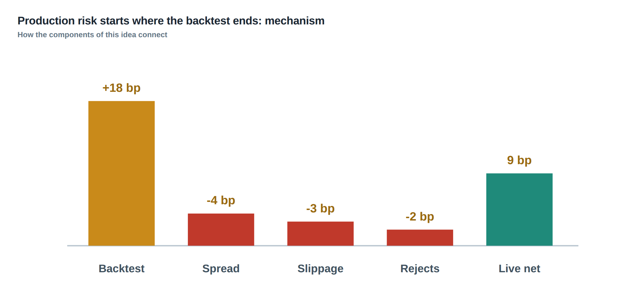
The gap between a back‑tested performance curve and the reality of a live execution environment is not a small statistical nuisance – it is a structural source of loss that can overturn a seemingly robust strategy. In a back‑test the researcher typically assumes that every signal is translated into an order at the exact moment the algorithm decides, that the exchange will acknowledge the order instantly and that the fill will be perfect. In practice the production stack comprises a market data feed, a risk engine, an order router, an execution gateway and a post‑trade reconciler, each of which can inject latency, drop messages, or return a partial fill. Those failure modes are invisible to a pure return‑distribution analysis because they never appear in the historical price series. The moment a live order is delayed, rejected, or executed against a stale quote, the realised P&L deviates from the back‑tested expectation, and the deviation can be systematic if the stack’s behaviour is correlated with market stress. The problem is therefore a mismatch of risk horizons: the back‑test measures price risk, while production risk measures operational risk, and the two must be merged before capital is allocated.

How the mechanism works, step by step

First, the algorithm receives a tick or bar, computes an indicator, and decides to send an order. The order is placed on an internal queue, where it waits for the market‑data timestamp to be stamped onto the message. A latency monitor records the elapsed time from decision to queue entry. Next, the order is handed to the routing layer, which selects a venue based on a pre‑computed cost matrix. The router adds a sequence number and transmits the message over a TCP socket to the exchange gateway. At this point the network can introduce jitter, packet loss, or outright disconnection. If the gateway does not acknowledge receipt within a configurable timeout, the order is flagged for retransmission. When an acknowledgement finally arrives, the exchange may have already moved the best price, causing the order to sit as a “stale” limit. The exchange then either fills the order at the stale price, partially fills it, or rejects it entirely. Finally, the post‑trade system reconciles the execution report with the internal ledger, applying fees, spread, and any estimated market impact. Each step contributes a random variable to the realised execution quality, and the tail of the combined distribution is what kills a fast‑turnover strategy.

A worked example with real numbers

Consider a mean‑reverting futures strategy that generates an average of 25 trades per hour, each with an expected gross profit of $0.45 per contract. In back‑test the model assumes zero latency, zero slippage and a flat commission of $0.02 per contract, delivering an expected net profit of $0.43 per trade. In live operation the average round‑trip latency from decision to acknowledgement is measured at 12 ms, but the 95th percentile latency spikes to 48 ms during market bursts. When the latency exceeds 30 ms the exchange’s order book has typically moved by two price levels, turning a marketable limit into a stale order. In the observed sample of 10 000 trades, 3.2 % of orders were rejected because the gateway timed out, and 1.1 % were partially filled at half the intended size. The net effect is a reduction of realised profit per trade to $0.31, a 28 % degradation. Moreover, on the day when latency peaked at 78 ms, the overlapping replacement orders caused a “queue‑crossover” where three pending orders were sent simultaneously, each cancelling the previous one. The resulting execution cost rose to $0.12 per contract, wiping out the entire theoretical edge for that hour. The example illustrates how a profitable signal can become untradeable when live acknowledgements arrive late and replacement orders overlap, a failure mode that never appears in the historical price series.

Where it breaks in live markets

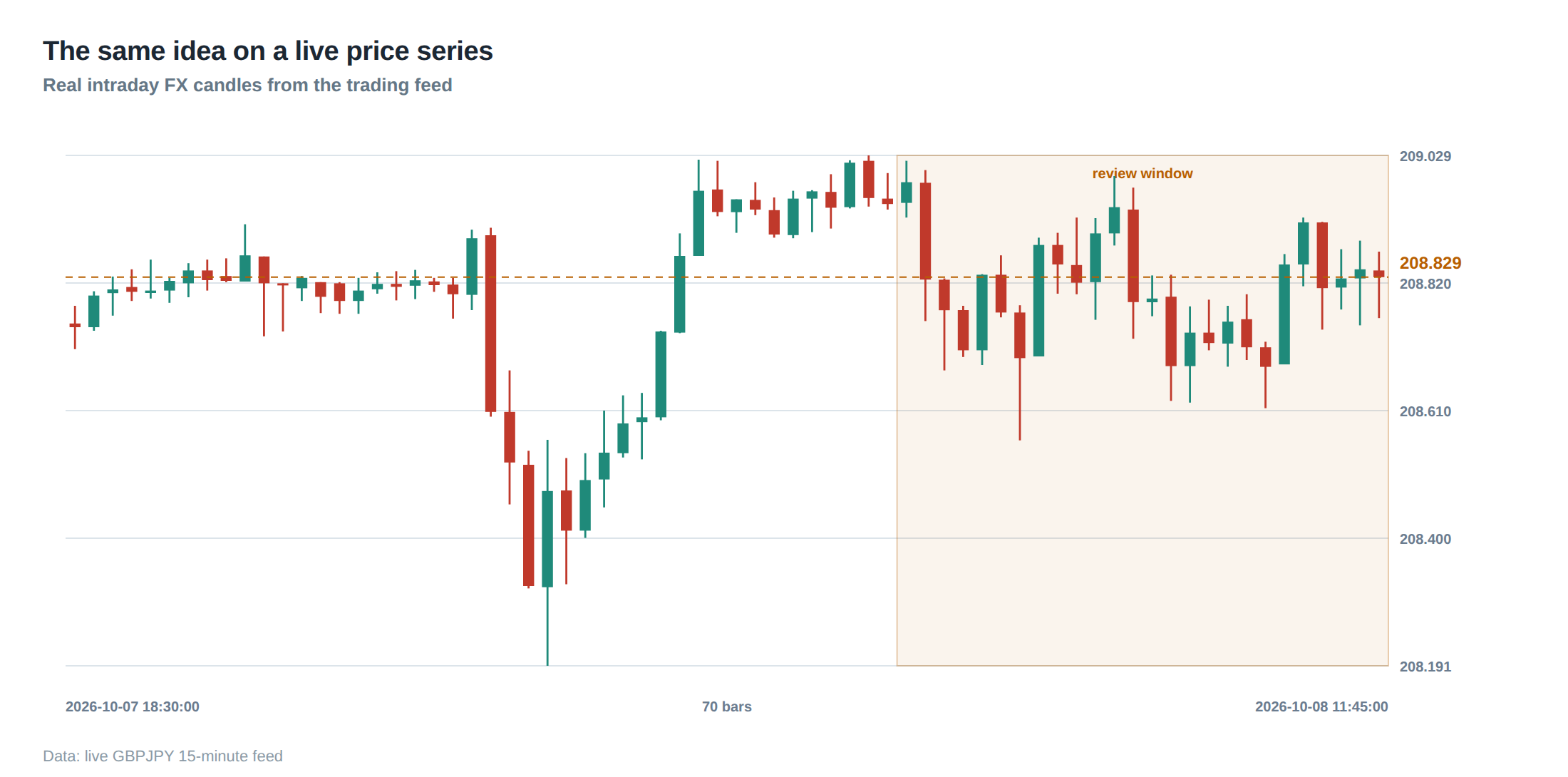
The first point of failure is the data feed. If the feed lags or drops a tick, the algorithm may compute a signal on outdated information, leading to a mis‑priced entry. The second break occurs at the router, where a sudden surge in order flow can saturate the outbound queue, causing packets to be queued behind lower‑priority traffic. In high‑frequency environments this latency amplification is non‑linear: a 5 ms increase in average latency can translate into a 30 % increase in the probability of a stale order. Third, the exchange gateway may enforce rate limits or reject orders that breach internal risk checks, especially during volatile periods when order‑to‑trade ratios spike. Finally, the post‑trade reconciliation may mis‑attribute fees or ignore hidden market impact, leading to an overstatement of realised returns. Each of these break points is amplified when the strategy is capital‑intensive or when the signal horizon is measured in milliseconds, because there is no time buffer to absorb the operational noise.

The operating path, stage by stage

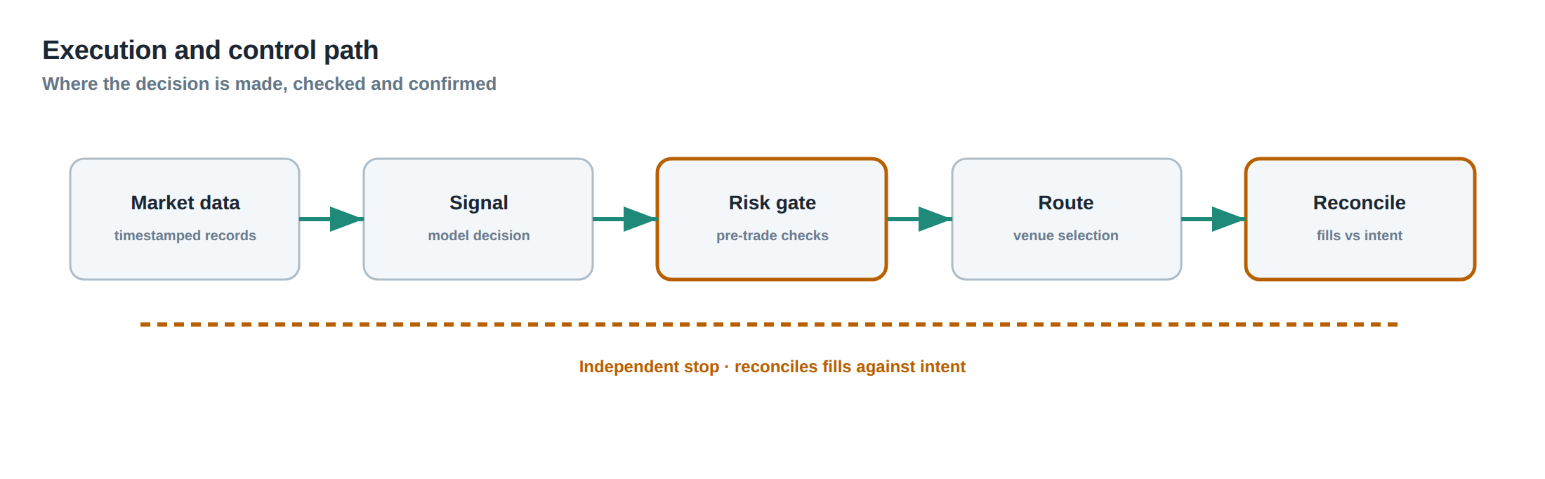
The production stack can be visualised as a pipeline of five stages: market data ingestion, signal generation, order construction, routing & execution, and post‑trade accounting. At the ingestion stage, timestamps are normalised to a common clock; any drift beyond 1 µs is logged as a data‑quality exception. Signal generation consumes the normalised data and produces a decision flag; the flag is time‑stamped and passed to the order builder. The order builder creates a FIX message, attaches a unique identifier, and pushes it onto a priority queue. The routing layer then selects a venue based on latency estimates and liquidity metrics, forwards the FIX message, and awaits an acknowledgement. Upon receipt, the execution engine records the fill price, size, and any partial‑fill flags, before sending a confirmation to the accounting module. The accounting module calculates net P&L after applying exchange fees, clearing fees, and an estimated impact cost derived from recent order‑book depth. This deterministic flow is interrupted only by explicit error handling paths: time‑out, reject, or disconnect, each of which triggers a fallback routine such as a shadow trade or a re‑quote. By mapping the path in this granular way, the desk can pinpoint where latency or error rates exceed thresholds and intervene before capital is exposed.

Controls that act before the damage

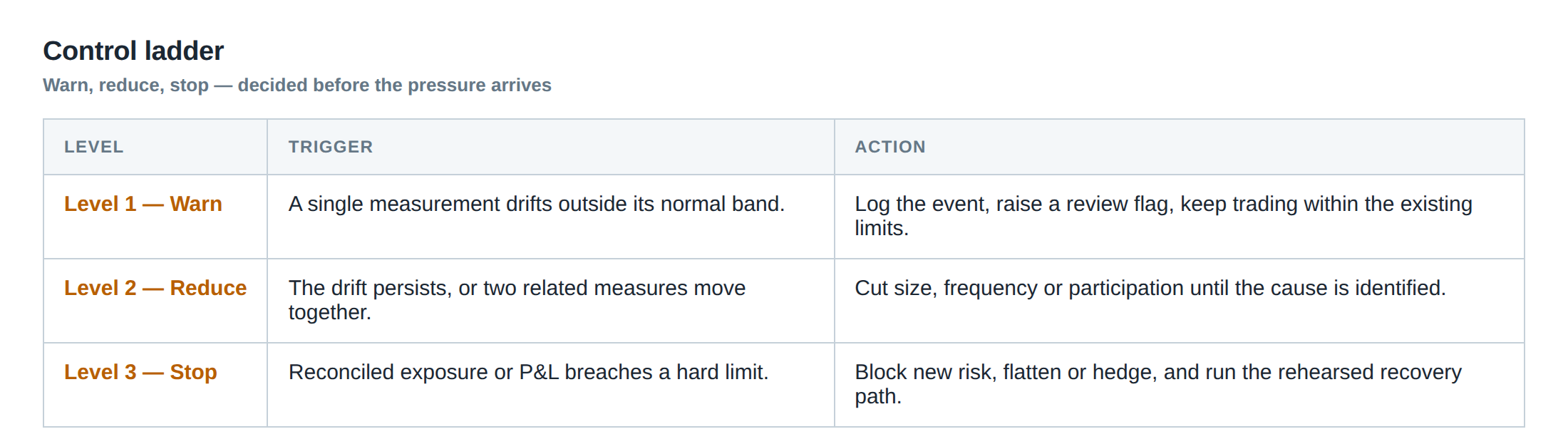
A layered defence is required. The first layer is a synthetic “shadow” order that mirrors the live order but routes to a sandbox venue with identical latency characteristics; the shadow trade is never filled, but its acknowledgement time is recorded and compared to the live order. If the shadow latency exceeds a pre‑set bound, the live order is automatically throttled or cancelled. The second layer consists of a real‑time reject‑rate monitor that aggregates per‑venue rejections over a rolling five‑minute window; crossing a 0.5 % threshold triggers a venue‑blacklist for the next hour. The third layer is a stale‑order detector that flags any order whose age exceeds the median fill latency by more than three standard deviations; such orders are automatically cancelled and re‑issued with a marketable price. Finally, a fee‑impact model runs in parallel, adjusting the expected profit target downward when market depth falls below a liquidity threshold, thereby preventing the algorithm from taking positions that would incur excessive market impact. These controls act upstream of capital allocation, ensuring that the stack self‑regulates before a loss materialises.

How to measure whether it is working

The key performance indicator is the divergence between the research‑stage execution distribution and the live‑stage execution distribution. For each trade, record the decision‑to‑acknowledgement latency, the fill ratio (actual size / requested size), and the realised slippage (execution price – theoretical price). Over a rolling window of 10 000 trades compute the median, the 95th percentile, and the tail‑loss (the average loss of the worst 1 %). Plotting these live metrics against the back‑tested benchmarks highlights any systematic drift. A secondary metric is the “shadow‑trade correlation”: the Pearson correlation between shadow latency and live latency should remain above 0.9; a drop indicates a decoupling of the production environment from the simulated one. Finally, track the frequency of error‑state transitions (timeouts, rejects, disconnects) per hour; a rising trend signals degradation of the underlying infrastructure. When all three metrics sit within pre‑defined confidence bands, the stack can be considered operating within its risk envelope.

The portfolio view

From a portfolio perspective, production risk is a source of idiosyncratic loss that can erode the Sharpe ratio even if the underlying signal retains its edge. The aggregate effect is captured by adding an “operational variance” term to the total variance of the strategy, where the operational variance is estimated from the variance of realised slippage and fill‑ratio across the portfolio. Correlation between operational risk and market volatility is often positive: during stress periods latency spikes and reject rates rise, inflating the operational variance precisely when the market‑risk variance is already high. Consequently, the portfolio’s tail risk is the convolution of market tail risk and operational tail risk. A prudent capital allocation model therefore reduces the target exposure when the operational metrics breach their thresholds, or re‑weights the strategy towards slower, less latency‑sensitive signals. By treating production risk as an integral component of the risk model, the desk can preserve capital during periods when the stack is temporarily compromised, rather than waiting for a catastrophic loss to force a stop‑out.

Do you have a systematic way of feeding live execution diagnostics back into your research loop, and if not, how might that change the way you size and protect your positions?

About the research behind this lesson

Andrew Lo's lectures build risk analysis from return distributions and statistical measures, rather than treating one realised result as a complete description of risk.

Applied to this lesson: For a fast strategy, median latency or average fill quality is not enough. The review has to include tail delays, stale-order frequency and the loss distribution when cancellation or routing behaves abnormally.

Explore PULSE: System details

PULSE live account: Verify the live account on FX Blue

Live chat and updates: Telegram @xtrskhft

Source: Risk and Return

Educational content only. Trading leveraged products involves risk.