October 9, 2026

What this problem really is

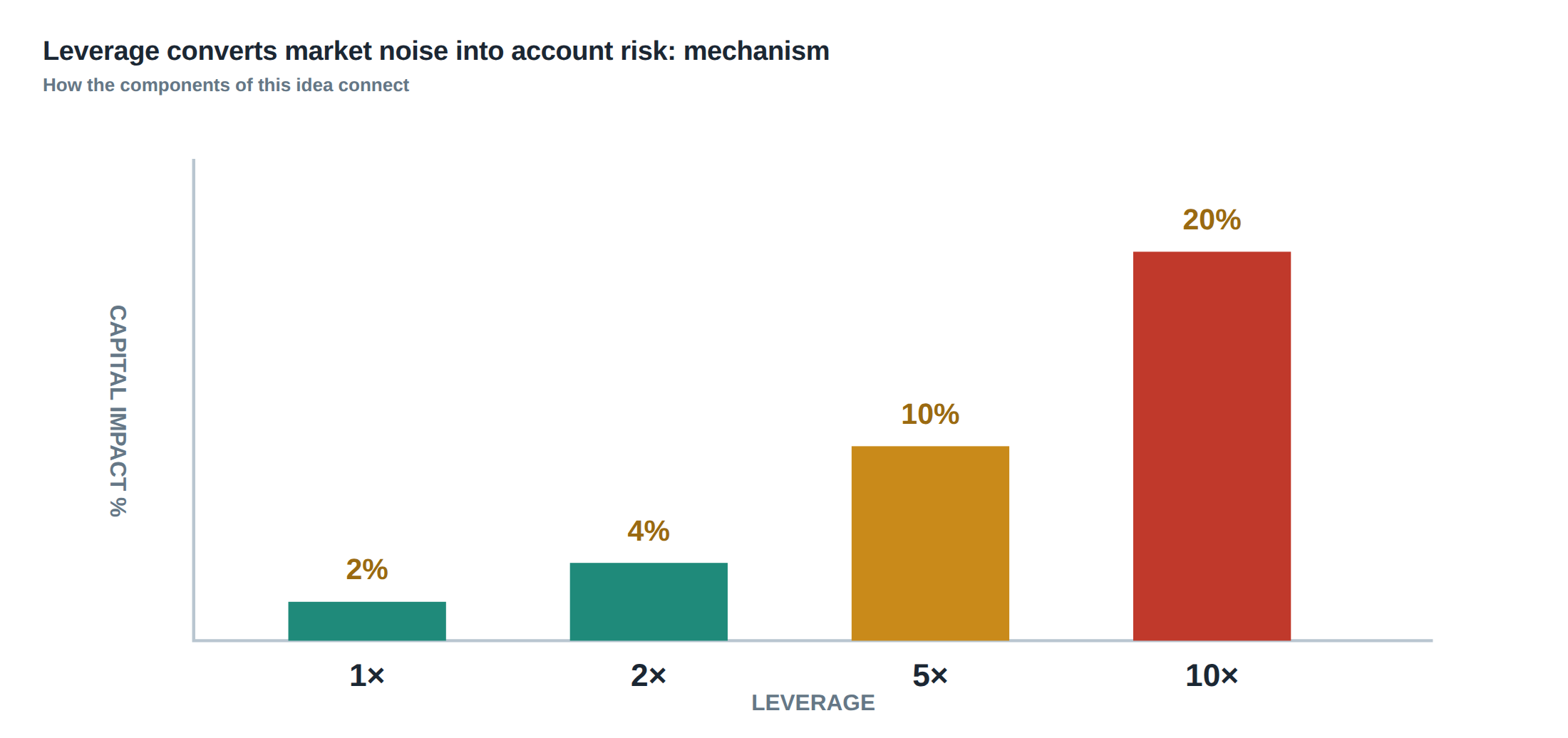
Leverage is often presented as a simple multiplier of profit potential, but the same multiplier magnifies every adverse price movement that the market throws at a position. When a trader treats the permitted margin as the sole sizing constraint, the distinction between gross exposure and the amount of capital truly at risk becomes blurred. The trader may be comfortable with a 10 % margin utilisation, yet a 2 % move against a five‑times levered position erodes ten percent of the underlying equity before commissions, slippage or financing costs are even considered. The gap between the notional size of the trade and the liquid capital that can be called upon in an emergency is the hidden source of ruin.

In practice the problem manifests as a cascade: a modest price swing triggers a margin call, the trader scrambles for cash, and the forced liquidation widens spreads, creating further losses. The process is deterministic, yet it is frequently masked by the allure of high Sharpe ratios that ignore the tail of the return distribution. The real issue is not the existence of leverage, but the failure to size exposure based on plausible adverse movements and the liquidity required to survive them.

How the mechanism works, step by step

The first step is the calculation of gross exposure, the notional amount of the position multiplied by the contract size. This figure is recorded in the risk engine but does not reflect the cash that would be depleted if the market moved sharply. The second step is the conversion of that exposure into a margin requirement, usually a percentage set by the clearing house. The trader then compares the required margin with the available cash and, if the ratio is acceptable, proceeds.

A third step introduces the dynamic component: as the market moves, the margin requirement is adjusted – often called variation margin. If the price drifts against the position, the required cash rises, and the trader must post additional funds. When the trader cannot meet the variation margin, the broker initiates a liquidation, which can be at unfavourable prices due to spread widening or order‑book gaps.

Finally, the feedback loop closes when the liquidation itself creates further market impact, widening spreads and deepening the price move, thereby feeding back into the margin calculation. The net effect is that a modest initial move can be amplified into a sizeable capital draw‑down, all because the sizing decision was anchored to a static margin ceiling rather than a realistic stress scenario.

A worked example with real numbers

Consider a prop desk that maintains a base capital of £1 million and elects to run a high‑frequency statistical arbitrage strategy with a leverage factor of five. The gross exposure therefore becomes £5 million. The clearing house requires an initial margin of 10 % of notional, i.e. £500 000, which comfortably sits within the desk’s cash buffer.

If the market experiences a sudden 2 % adverse move – perhaps due to an unexpected macro announcement – the notional loss on the £5 million exposure is £100 000. Because the position is levered five times, the loss represents ten percent of the original £1 million capital before any transaction costs are applied. The variation margin call would demand an additional £100 000 to restore the required 10 % coverage, instantly eroding the liquidity reserve.

Assuming an average execution cost of 5 bps and a spread widening of 10 bps during the stress moment, the total cost adds another £75 000 to the loss, pushing the capital hit to roughly £175 000, or 17.5 % of the original equity. The example demonstrates how a seemingly small price move, when magnified by leverage, can convert market noise into a material risk event that threatens the whole account.

Where it breaks in live markets

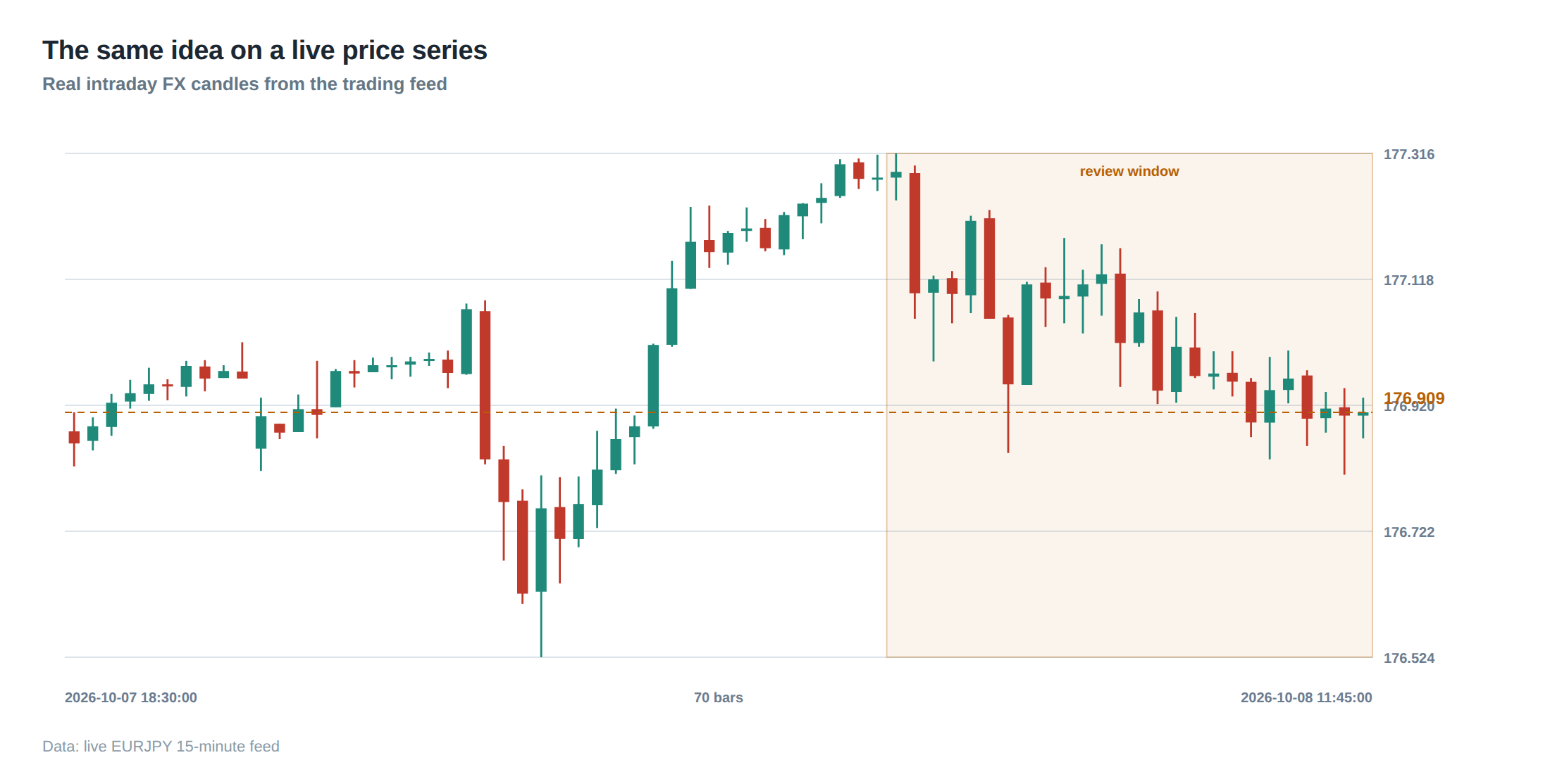
In live trading the idealised assumptions of continuous pricing and frictionless execution rarely hold. Gaps can appear when the market opens after a news shock, and the order book may be thin, causing the best bid‑ask to shift dramatically within milliseconds. Spread expansion is not a linear function of volatility; it can double or triple in the seconds surrounding a macro release.

Liquidity that looks ample on paper may evaporate when multiple desks simultaneously seek to meet margin calls, creating a race to the bottom. Moreover, the margin algorithms of clearing houses can change abruptly – for example, moving from a 10 % to a 15 % requirement in response to heightened systemic risk – forcing a sudden cash outflow. When a trader has sized positions solely on the maximum permitted margin, these abrupt changes can trigger a cascade of forced liquidations that the original risk model never anticipated.

The final breakdown often occurs at the intersection of three forces: a price gap that exceeds the assumed volatility buffer, a spread that widens beyond the expected transaction cost, and a margin requirement that spikes just as the cash buffer is depleted. The confluence of these factors transforms ordinary market noise into a capital‑draining event.

The operating path, stage by stage

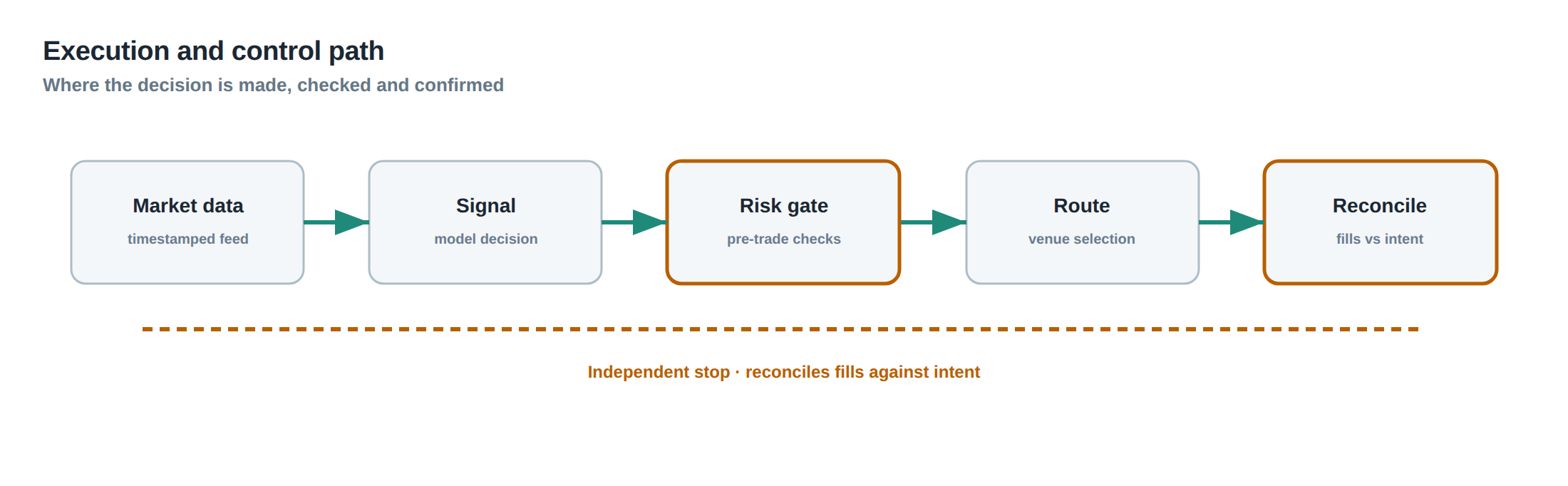
Stage one begins with the pre‑trade check, where the risk engine evaluates the intended notional against both the static margin ceiling and a stress‑scenario buffer derived from historical tail movements. Stage two involves the allocation of a dedicated liquidity reserve, separate from the trading capital, earmarked for variation margin and emergency hedging.

Stage three is the real‑time monitoring loop. Market data feeds feed the engine with price, depth and volatility metrics; any deviation beyond the pre‑set stress thresholds triggers an alert. The system then assesses the current utilisation of the liquidity reserve and, if necessary, initiates a partial unwind of the most correlated positions to free cash without dramatically increasing overall exposure.

Stage four is post‑trade reconciliation, where the realised P&L, the variation margin posted, and the actual execution costs are compared against the modelled expectations. Discrepancies are logged, and the stress parameters are recalibrated for the next trading day. This staged approach ensures that leverage is continually reconciled with the true amount of capital at risk, rather than being left to a single static margin check.

Controls that act before the damage

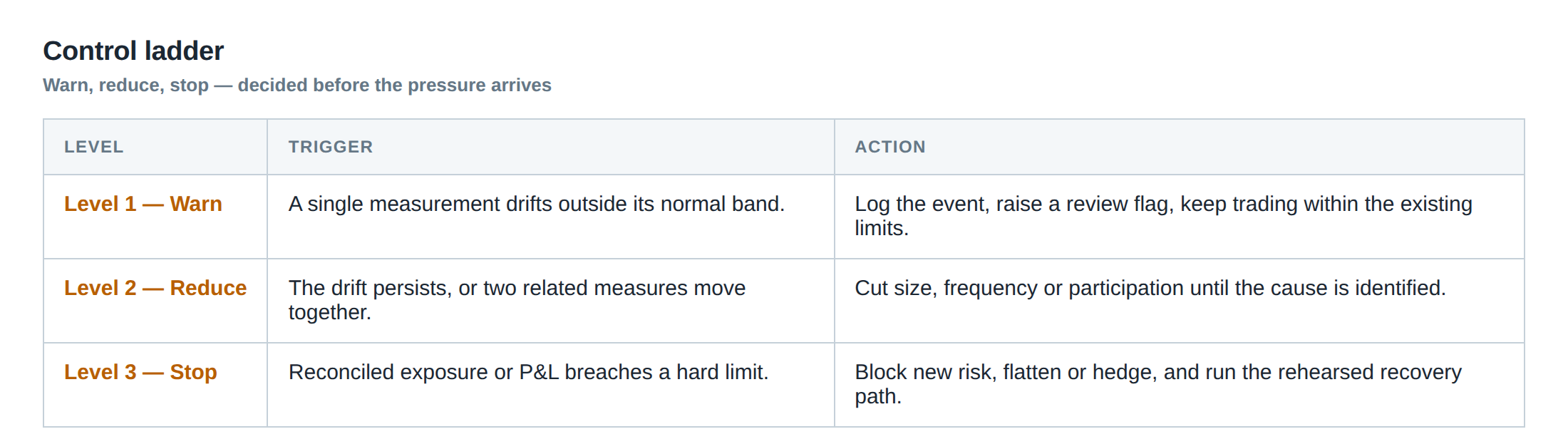
A robust control framework places hard limits on the aggregate leverage across all correlated positions, not merely on each individual trade. By capping the net exposure of a basket of statistically linked instruments, the desk prevents the inadvertent stacking of risk that would otherwise be hidden behind a collection of apparently modest positions.

Liquidity buffers are enforced through a “margin ladder” that requires a proportion of cash to be locked away in a non‑trading account. The ladder steps rise with the level of exposure: a 3‑times levered position must keep 15 % of capital in reserve, a 5‑times levered position 25 %, and so on. These buffers are automatically deducted from the available cash for new trades, ensuring that the desk never over‑commits its liquid resources.

Another pre‑emptive control is the use of dynamic stop‑loss bands that are calibrated to the worst‑case gap observed in the last 250 trading days, rather than to a simple standard‑deviation measure. When price breaches the band, the system executes a market‑or‑limit order to reduce exposure before the margin call escalates. Together, these controls create a multi‑layered safety net that acts well before any capital loss materialises.

How to measure whether it is working

Effectiveness is gauged by tracking the frequency and magnitude of variation‑margin calls relative to the size of the liquidity reserve. A declining ratio indicates that the reserve is sufficient to absorb typical stress events. Additionally, the desk should monitor the realised tail loss distribution – the empirical quantiles of daily P&L – and compare them against the modelled stress scenarios used for sizing.

Another key metric is the “leverage utilisation factor”, defined as the ratio of gross exposure to the sum of capital at risk and the liquidity buffer. When this factor remains below the pre‑defined ceiling across the trading day, the control regime can be considered functional. Finally, the incidence of forced liquidations due to margin shortfalls should be logged; a near‑zero count over a statistically significant period suggests that the pre‑trade sizing and liquidity‑reserve policies are succeeding.

Regular back‑testing against out‑of‑sample market shocks – for example, the price action surrounding a sudden rate decision – provides an additional sanity check. If the simulated losses under those conditions stay comfortably within the allocated reserve, the measurement framework can be deemed robust.

The portfolio view

From a portfolio perspective, leverage must be treated as a collective property rather than a series of independent levers. Correlation matrices derived from high‑frequency return data reveal hidden clusters of exposure that can amplify a single market move into a multi‑instrument loss. By aggregating the gross exposure of each cluster and applying a common stress factor, the desk can enforce a portfolio‑wide leverage ceiling that respects the true risk of simultaneous adverse moves.

Liquidity considerations also become portfolio‑wide. The total cash required for variation margin across all positions must be less than the sum of the dedicated liquidity buffer and the expected cash inflow from any scheduled hedging activities. If a subset of the portfolio is earmarked for hedging, the timing of those cash flows must be synchronised with the potential margin calls to avoid a liquidity crunch.

In the end, the discipline of sizing exposure from plausible adverse movement and available liquidity, rather than from the maximum permitted margin, creates a more resilient trading operation. It aligns the theoretical leverage with the practical capacity to meet cash obligations, thereby converting market noise from a source of hidden danger into a manageable element of the risk budget.

Do you currently size your positions based on a realistic stress scenario and a dedicated liquidity reserve, or do you still rely primarily on the static margin ceiling set by the exchange?

About the research behind this lesson

Andrew Lo's lectures build risk analysis from return distributions and statistical measures, rather than treating one realised result as a complete description of risk.

Applied to this lesson: For a fast strategy, median latency or average fill quality is not enough. The review has to include tail delays, stale-order frequency and the loss distribution when cancellation or routing behaves abnormally.

Explore PULSE: System details

PULSE live account: Verify the live account on FX Blue

Live chat and updates: Telegram @xtrskhft

Source: Risk and Return

Educational content only. Trading leveraged products involves risk.