October 9, 2026

What this problem really is

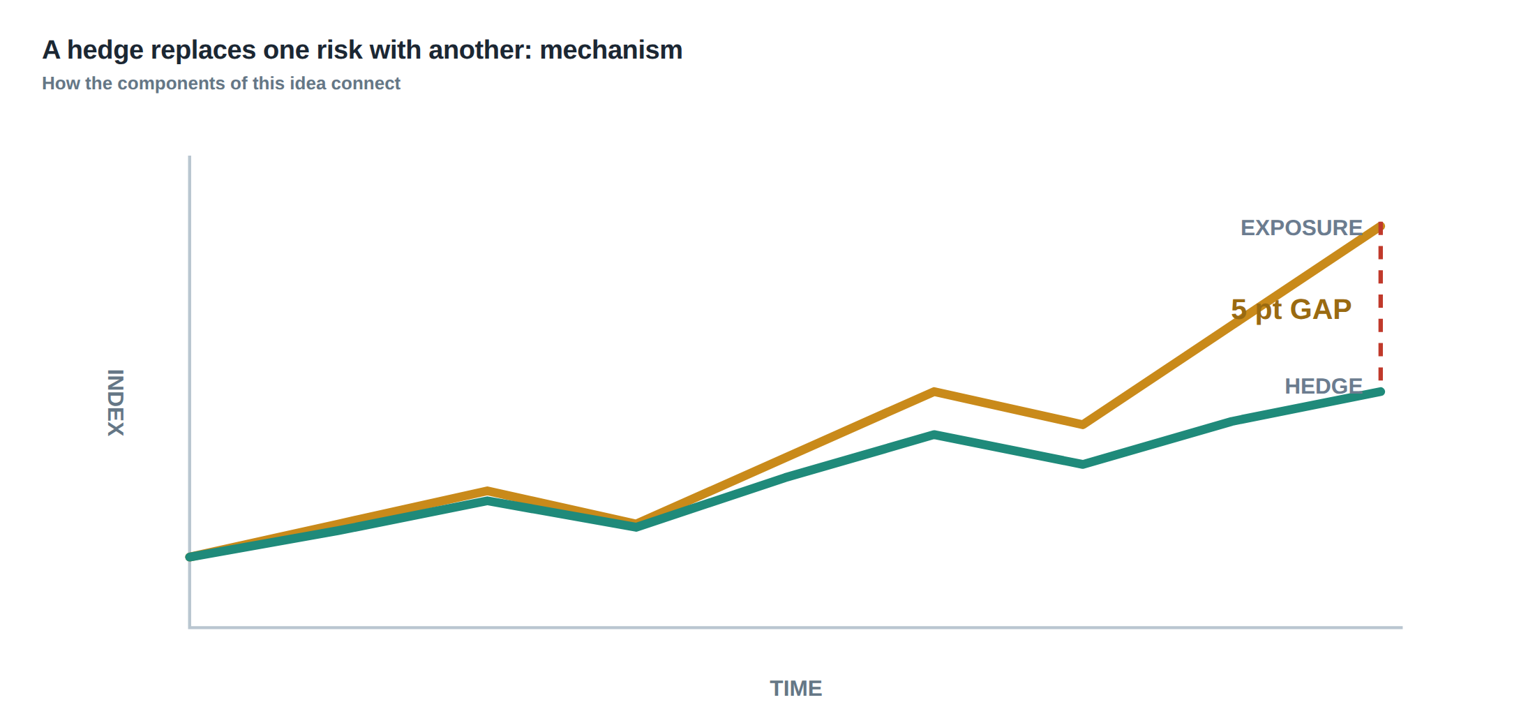
When a desk decides to hedge a position it is tempting to think of the hedge as a simple subtraction: the exposure to the original factor disappears and the portfolio is left neutral. In practice the hedge is a contract that moves with the underlying factor only imperfectly. The residual that remains is called basis risk, and it is only one of several hidden layers. Execution risk appears when the hedge cannot be entered at the quoted price, liquidity risk when the market cannot absorb the required size without moving the price, and model risk when the statistical relationship that underpins the hedge is misspecified or breaks down in stress. All of these risks are present even before the hedge is placed; they become visible only when the market moves, when funding costs accrue, or when the hedge has to be rolled. The core thesis, therefore, is that hedging reduces a chosen exposure but inevitably substitutes it with a suite of other, often less obvious, risks that must be quantified and managed.

The factor being hedged can be a commodity price, a foreign‑exchange rate, an equity index, or a more abstract statistical driver such as a principal component of a basket of securities. Defining the factor precisely matters because the hedge ratio, the timing of roll, and the financing cost all depend on the exact contract specifications. A mis‑specification— for example treating a futures contract as a perfect proxy for a spot exposure without adjusting for the cost‑of‑carry— introduces a deterministic drift that will erode P&L over time. The desk must therefore start by stating the exposure in terms of a measurable variable, e.g. “the portfolio is long 10 000 EUR of 3‑month LIBOR exposure” rather than a vague “interest‑rate risk”.

The literature on risk measurement stresses that a single realised outcome cannot capture the full distribution of possible results. Return distributions, tail moments and conditional expectations give a richer picture of the risk that the hedge is supposed to eliminate. In a fast‑moving strategy, focusing only on median latency or average fill quality is insufficient; the tail of the latency distribution, the frequency of stale orders and the loss distribution when routing behaves abnormally are equally important. Those same statistical tools should be applied to the hedge itself: the distribution of hedge error, the probability that the hedge will be partially filled, and the expected cost of financing the hedge over its life all belong in the risk‑budget.

How the mechanism works, step by step

The first step is to identify the risk factor and to choose a proxy instrument that is liquid enough to trade in the required size. The proxy may be a futures contract, an exchange‑traded fund, a total‑return swap or a bespoke forward. Once the proxy is chosen, the hedge ratio is calculated, usually by linear regression of historic returns of the underlying factor against the proxy. The regression coefficient gives the minimum‑variance hedge ratio, while the standard error of that coefficient quantifies the uncertainty in the hedge size. A desk that ignores the confidence interval will often under‑ or over‑hedge, exposing the portfolio to residual directional risk.

The second step is to translate the hedge ratio into a concrete order size, adjusting for contract specifications such as tick size, multiplier and margin requirement. At this point the financing cost of the hedge must be added: futures require daily margin, swaps involve collateral posting, and forwards may need upfront cash. The cost of carry— the difference between the risk‑free rate and the implied financing embedded in the proxy— is a deterministic drift that will affect the hedge’s performance over the holding period.

The third step is execution. The order is routed, possibly split across venues to minimise market impact, and a limit price is set based on the prevailing bid‑ask spread. Execution risk is captured by the probability that the order is only partially filled or that the fill occurs at a worse price than expected. If the market is thin, the order itself may move the price, creating slippage that adds to the hedge error.

The final step is monitoring. As time passes, the basis between the underlying factor and the hedge evolves. The desk must track the spread, calculate the realised hedge error, and decide whether to re‑balance or to roll the hedge into a later‑dated contract. Financing costs continue to accrue, and the roll itself may involve a cost if the forward curve is not flat. All of these elements feed back into the risk model, updating the hedge‑ratio uncertainty and informing the next iteration.

A worked example with real numbers

Consider a desk that is long €10 million of a 3‑month Euribor exposure, realised through a portfolio of floating‑rate notes. The chosen hedge is a Euro‑dollar futures contract that tracks the 3‑month USD LIBOR rate, which historically correlates 0.92 with Euribor. A regression over the past 250 business days yields a hedge ratio of 0.95 with a standard error of 0.04. The desk therefore decides to sell 9.5 contracts (each contract representing €1 million notional) to offset the Euribor exposure, accepting a 5 % residual hedge error as a trade‑off for liquidity.

The financing cost of the futures position is calculated as the difference between the Euro‑area risk‑free rate (0.25 % p.a.) and the implied financing in the Euro‑dollar contract (0.30 % p.a.), giving a net cost of 0.05 % per annum, or €5 000 for the three‑month horizon. Roll cost is estimated from the forward curve: the June contract trades at a spread of 2 bps over the spot rate, while the September contract trades at 3 bps, implying a roll cost of 1 bp, or €1 000 on the notional.

During a calm market the hedge reduces the portfolio’s directional variance by roughly 85 %, as the proxy tracks Euribor closely. However, in a stress episode— for instance a sudden Euro‑dollar funding shock— the correlation collapses to 0.60 and both spreads widen: the Euribor‑LIBOR spread widens from 5 bps to 35 bps, while the futures bid‑ask widens from 1 bp to 8 bps. The hedge then delivers only a 30 % variance reduction, and the combined basis and execution cost amounts to a loss of €45 000, far exceeding the expected financing and roll costs. The example demonstrates that a statistically sound hedge can still fail when the underlying relationship breaks, and that the tail of the hedge‑error distribution must be incorporated into the risk budget.

If the order to sell 9.5 contracts is only partially filled— say 6 contracts are executed before the market moves— the desk faces an incomplete hedge. The residual exposure of €4 million now carries the full Euribor risk, and the realised hedge error widens dramatically. The desk must therefore have a contingency plan: either a pre‑approved secondary venue to complete the order, or a dynamic re‑balancing rule that scales the hedge up as liquidity re‑appears. The plan should also specify the maximum acceptable fill‑rate shortfall before the hedge is deemed rejected and the exposure is re‑allocated.

Where it breaks in live markets

The first point of failure is the assumption that the statistical relationship between the factor and the proxy is stationary. In reality, correlations are regime‑dependent; macro‑economic shocks, policy changes or market micro‑structure events can cause abrupt decoupling. When the correlation falls, basis risk spikes and the hedge no longer offsets the intended exposure. The second failure mode is execution under stress. Liquidity can evaporate within minutes, causing the order book to thin and spreads to widen dramatically. A limit order placed at the pre‑trade mid‑price may never be hit, leaving the hedge incomplete while the underlying moves.

Financing risk becomes acute when the funding curve steepens unexpectedly. A hedge that was originally cheap to carry can suddenly become expensive, eroding the P&L even if the basis remains narrow. Roll risk is another hidden source of loss: if the forward curve is steep, rolling a futures position into a later contract can generate a sizeable cost that dwarfs the expected benefit of the hedge. Finally, model risk appears when the regression used to estimate the hedge ratio does not capture non‑linearities or tail dependencies; the standard error may understate the true uncertainty, leading the desk to believe the hedge is more precise than it actually is.

The operating path, stage by stage

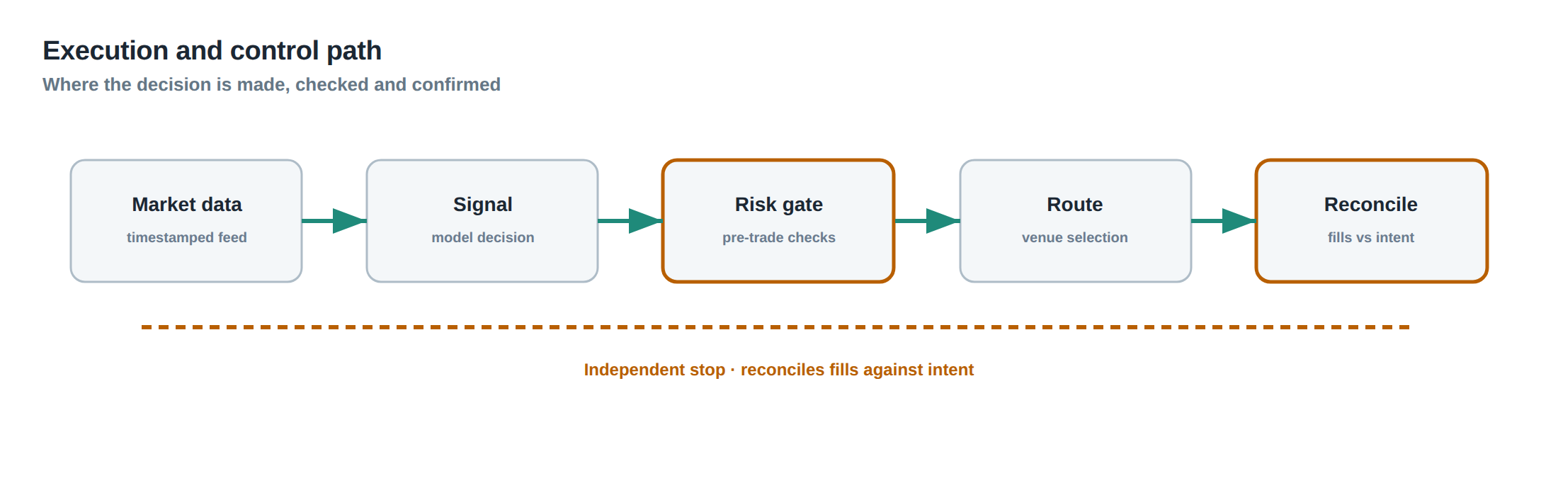
Stage 1: Exposure identification. The desk quantifies the factor in monetary terms, for example €10 million of Euribor exposure, and records the measurement horizon (e.g. 3 months). Stage 2: Proxy selection and ratio estimation. Historical data are cleaned, outliers are examined, and a regression is run to obtain the hedge ratio and its confidence interval. Stage 3: Order construction. The hedge size is converted into contract units, financing and roll costs are added, and a limit price is set based on current market depth. Stage 4: Execution monitoring. Real‑time market data are compared to the order book; any deviation from the expected fill rate triggers an alert. Stage 5: Post‑trade reconciliation. The realised hedge error, financing expense and any slippage are recorded, and the basis is updated. Stage 6: Review and roll. As the contract approaches expiry, the desk evaluates whether the basis has widened beyond a pre‑defined threshold and decides whether to roll, unwind or augment the hedge.

Controls that act before the damage

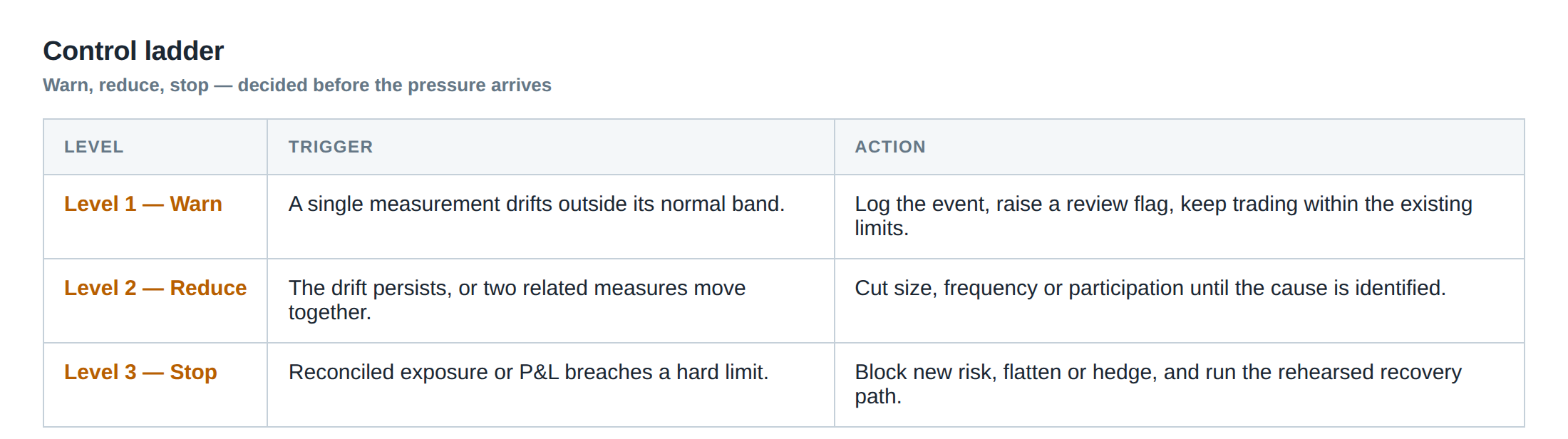
The first line of defence is a pre‑trade model validation that checks the stability of the hedge‑ratio estimate. The model must produce not only a point estimate but also a confidence band; if the standard error exceeds a set threshold (for example 5 % of the ratio) the trade is blocked and escalated. The second control is a liquidity screen that inspects the depth of the proxy market across multiple venues; a minimum depth of €2 million at the target price must be present before the order is submitted. A third control is a financing‑cost guard that compares the implied financing of the proxy to the desk’s internal funding rate; any excess beyond a defined limit aborts the trade. Finally, an execution‑risk monitor watches the order flow in real time; if the fill‑rate falls below 80 % within the first five minutes, the system automatically cancels the remainder and raises a ticket for manual intervention. These controls are arranged in a ladder‑like hierarchy, with each rung preventing the trade from progressing if its criteria are not met.

How to measure whether it is working

Effectiveness is measured by the reduction in the variance of the hedged exposure relative to the unhedged one, adjusted for the cost of the hedge. The realised hedge error series is examined for its mean, standard deviation and tail quantiles (e.g. 99 % VaR). A useful metric is the “cost‑adjusted hedge efficiency”, defined as the variance reduction divided by the sum of financing, roll and execution costs. The distribution of this metric over rolling windows highlights periods when the hedge is under‑performing. Additionally, the frequency and magnitude of basis spikes are tracked; a high spike‑frequency indicates that the proxy is losing relevance. Finally, the proportion of orders that are partially filled or rejected is recorded as an execution‑quality KPI. Together these statistics give a comprehensive view of whether the hedge is delivering the intended risk mitigation.

The portfolio view

When the hedge is embedded in a larger portfolio, its residual risks interact with other positions. Basis risk may be offset by other hedges that use different proxies, creating a net‑zero exposure to the same factor. Conversely, liquidity risk can become systemic if multiple desks simultaneously attempt to unwind similar contracts, amplifying market impact. The portfolio‑level risk model must therefore treat each hedge as a separate risk factor with its own volatility, correlation and cost structure. Aggregating the cost‑adjusted hedge efficiencies across the portfolio yields a macro‑level assessment of how much risk is being transferred from market exposure to operational and model exposure. The desk should allocate capital not only on the basis of expected return but also on the basis of the residual risk budget that remains after accounting for all hedge‑related risks.

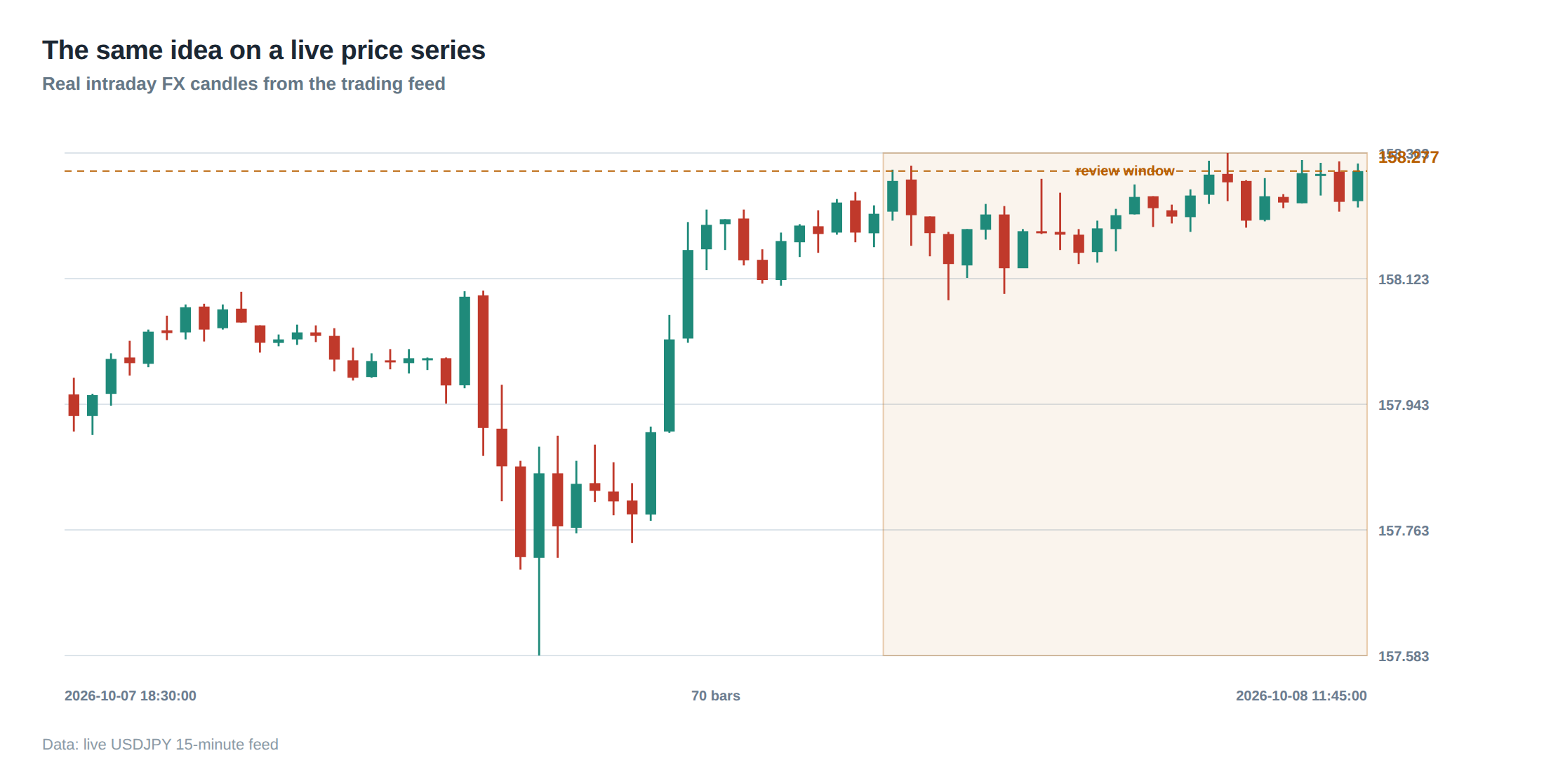
In summary, a hedge is never a pure subtraction of risk; it is a transformation that replaces one exposure with a mixture of basis, execution, liquidity and model risks, each of which must be quantified, monitored and controlled. By following a disciplined, stage‑by‑stage process, by embedding robust pre‑trade controls, and by measuring performance with cost‑adjusted efficiency metrics, a prop‑trading desk can ensure that the hedge adds value rather than hidden danger.

Do you have a concrete plan for how your desk will detect and react to a sudden breakdown in the correlation that underpins your most heavily used hedge?

About the research behind this lesson

Andrew Lo's lectures build risk analysis from return distributions and statistical measures, rather than treating one realised result as a complete description of risk.

Applied to this lesson: For a fast strategy, median latency or average fill quality is not enough. The review has to include tail delays, stale-order frequency and the loss distribution when cancellation or routing behaves abnormally.

Explore PULSE: System details

PULSE live account: Verify the live account on FX Blue

Live chat and updates: Telegram @xtrskhft

Source: Risk and Return

Educational content only. Trading leveraged products involves risk.