October 16, 2026

What this problem really is

The moment a back‑test finishes, the analyst hands the strategy over to a live execution stack. In the back‑test the only uncertainties are the price series, the sampling frequency and the modelled transaction cost. In the live stack every component – market data feed, order gateway, risk engine, connectivity to the exchange – introduces a new stochastic element that is invisible to the historical return distribution. Production risk is therefore the collection of failure modes that are not captured by the back‑tested profit‑and‑loss curve: delayed acknowledgements, partial fills, order rejections, network disconnects, stale quotes and the non‑linear impact of real‑world fees. When any of these events occur, the realised path of the strategy diverges from the simulated path, and the realised distribution of returns can acquire heavy left‑hand tails that were never present in the research data. The problem is not a lack of data, but a mismatch between the abstracted, friction‑free environment of the back‑test and the messy, asynchronous reality of a production trading system.

How the mechanism works, step by step

First, the research engine generates a list of intended child orders, each stamped with a target price, quantity and a deadline by which the order must be acknowledged. The order management system (OMS) translates these intents into FIX messages, attaches a sequence number and forwards them to the gateway. The gateway queues the messages, attaches a local timestamp and pushes them across the network. On the exchange side the order book receives the message, validates it against market rules and either acknowledges, rejects or silently drops it if the market data feed is out of sync.

If the acknowledgement arrives within the expected latency envelope, the OMS marks the order as live and monitors fill events. If the acknowledgement is delayed beyond the deadline, the OMS may cancel the order and issue a replacement. In a fast‑moving market, a replacement order can be submitted while the original is still pending, creating overlapping exposure. The exchange may then fill only part of the first order before the second one arrives, leaving a residual position that the strategy never intended to hold.

All of these steps generate a sequence of timestamps, status codes and fill quantities that must be reconciled with the original intent. The reconciliation is where the production‑risk profile is formed: each deviation from the intended order flow adds a stochastic term to the realised P&L that is not present in the back‑tested return series.

A worked example with real numbers

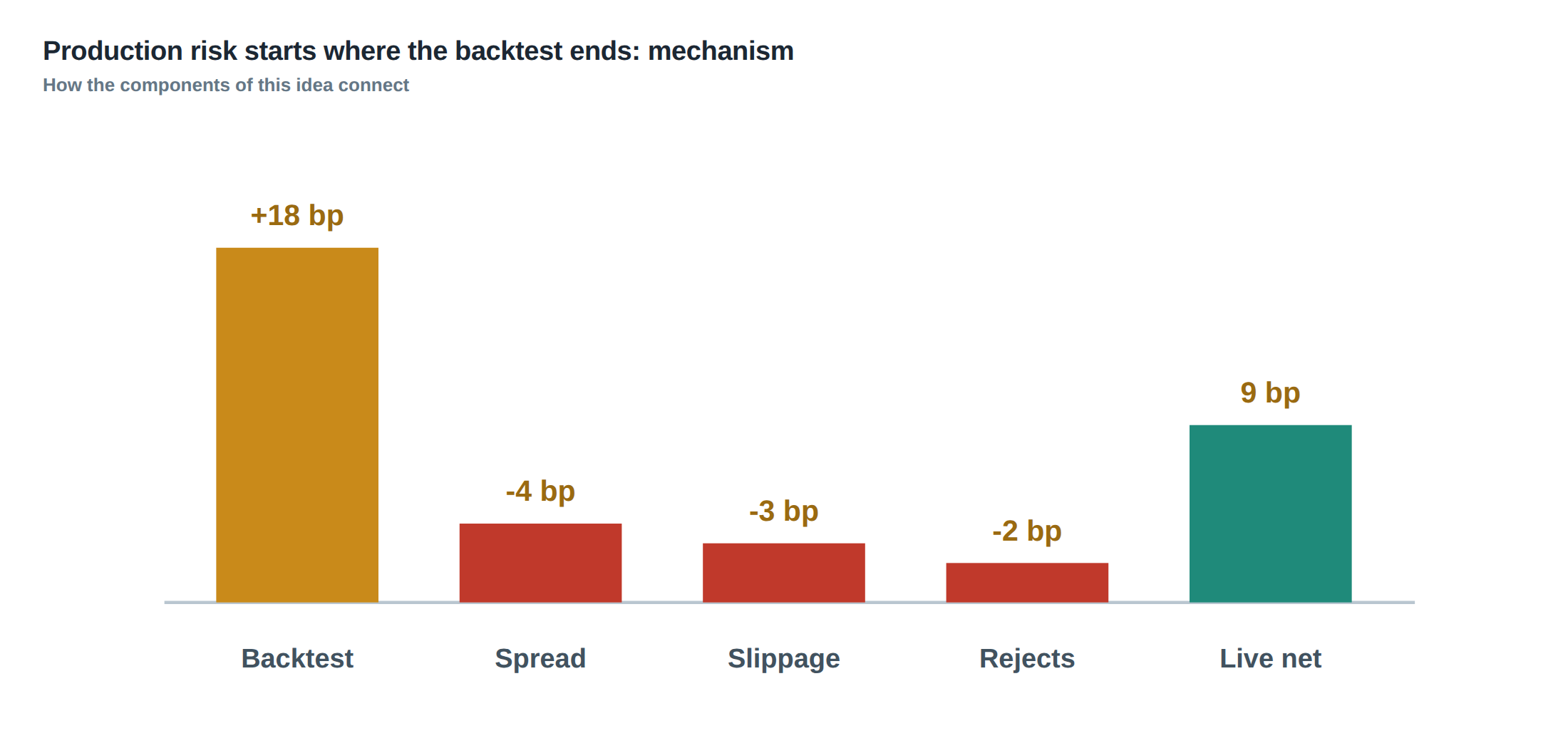
Consider a mean‑reversion signal that, on a 1‑second bar, predicts a 0.5 % price move to the upside with a win probability of 55 %. In the back‑test the signal generates 10 000 trades over a six‑month horizon, each trade having an expected gross profit of $0.50 after a flat commission of $0.02 and an assumed slippage of $0.01. The simulated Sharpe ratio is 2.1, and the distribution of daily returns shows a negligible left tail.

In production the same signal is executed on a low‑latency venue. The median round‑trip latency from order submission to acknowledgement is 30 ms, but the 99th percentile latency spikes to 210 ms during periods of network congestion. The OMS is configured to cancel and replace any order that has not been acknowledged within 100 ms. On a particular 5‑minute burst the following sequence occurs:

At 09:30:12.000 the OMS sends a market‑able limit order for 10 000 shares at $100.05. The exchange receives the message at 09:30:12.030 and acknowledges at 09:30:12.045 – within the median envelope. At 09:30:12.080 the OMS receives a market data update indicating that the best ask has moved to $100.07, and the strategy decides to improve the price. It issues a replacement order for 10 000 shares at $100.07, cancelling the first order. Because of a transient congestion event, the acknowledgement for the cancellation arrives only at 09:30:12.300, well beyond the 100 ms deadline. The replacement order is already in the gateway queue and is transmitted at 09:30:12.110, reaching the exchange at 09:30:12.140.

The exchange now holds two live orders: the original at $100.05 (still active because the cancellation never arrived) and the replacement at $100.07. The market moves against the position, the best bid falls to $99.95, and the original order is filled partially for 4 000 shares at $100.05. The replacement is never filled. The strategy ends the bar with an unintended long exposure of 4 000 shares, which is subsequently liquidated at $99.90, incurring a loss of $0.15 per share, i.e. $600 total.

If the back‑test had assumed perfect acknowledgements, the same bar would have produced a profit of $5 (10 000 × $0.0005). The single latency tail event has therefore erased the expected profit and added a sizeable loss, turning a profitable signal into an untradeable one for that interval.

Where it breaks in live markets

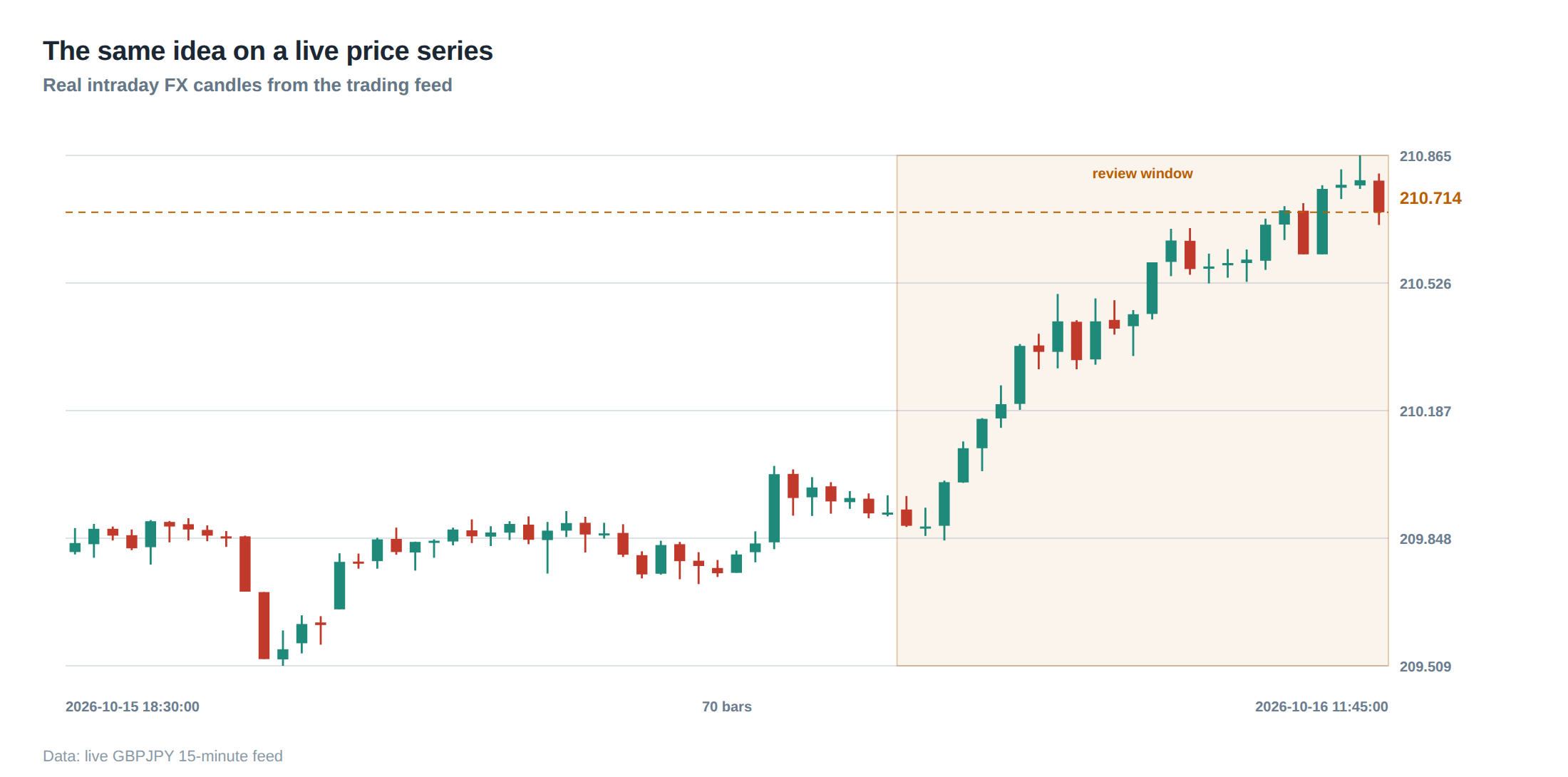
The first breach typically occurs when the latency distribution widens beyond the range observed in the research environment. A strategy that tolerates a 30 ms median delay cannot survive a 200 ms tail without adjusting its order‑lifecycle logic. The second breach is the interaction between order replacement logic and exchange throttling. Exchanges often impose per‑second rate limits; when a flood of cancellations and new orders is generated, the gateway may be forced to drop messages, leading to silent rejects that the OMS never records.

A third failure mode is stale market data. If the data feed lags the exchange by more than a few milliseconds, the strategy may calculate a price that is already obsolete, causing orders to be placed inside the spread or beyond the best price level. The resulting fills are either partial or executed at a worse price, inflating slippage beyond the assumed $0.01 per share.

Finally, fee structures that depend on order type, venue or executed volume can introduce a non‑linear cost curve. In the back‑test a flat $0.02 commission per share is applied, but in production the exchange may charge a maker‑taker fee that rises sharply once the daily volume threshold is crossed. The hidden increase in cost appears only after the strategy has already generated a series of trades, eroding the tail of the return distribution.

The operating path, stage by stage

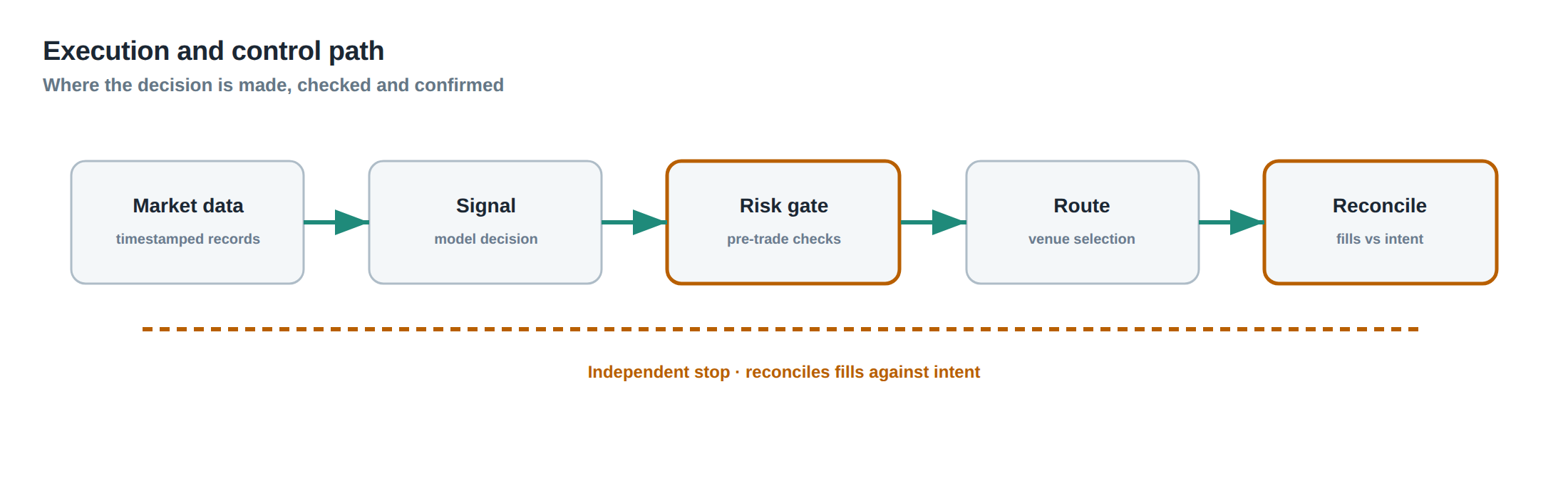
The production stack can be divided into four logical stages. Stage 1 is the signal generation module, which consumes a cleaned price feed and outputs a list of trade intents. Stage 2 is the order translation layer, which maps intents to FIX messages, attaches timestamps and forwards them to the gateway. Stage 3 is the connectivity layer, comprising the network stack, the exchange gateway and any intermediate broker‑side risk checks. Stage 4 is the execution feedback loop, which receives acknowledgements, fill reports and market data updates, reconciles them with the original intents and updates the position book.

Each stage introduces its own stochastic latency and error distribution. In Stage 1 the only source of randomness is the stochastic nature of the price series; in Stage 2 the serialization of messages adds a deterministic but non‑zero processing delay. Stage 3 is where most tail events originate: packet loss, queue overflow, and exchange‑side throttling can all produce out‑of‑order or missing acknowledgements. Stage 4 must cope with partial fills and stale quotes, and its reconciliation logic determines whether a missed acknowledgement becomes a cancellation, a replacement or a silent loss.

By visualising the stack as a pipeline, one can identify where buffers should be placed, where time‑outs need to be tightened and where redundancy (e.g. dual network paths) can be injected to reduce the probability of catastrophic latency spikes.

Controls that act before the damage

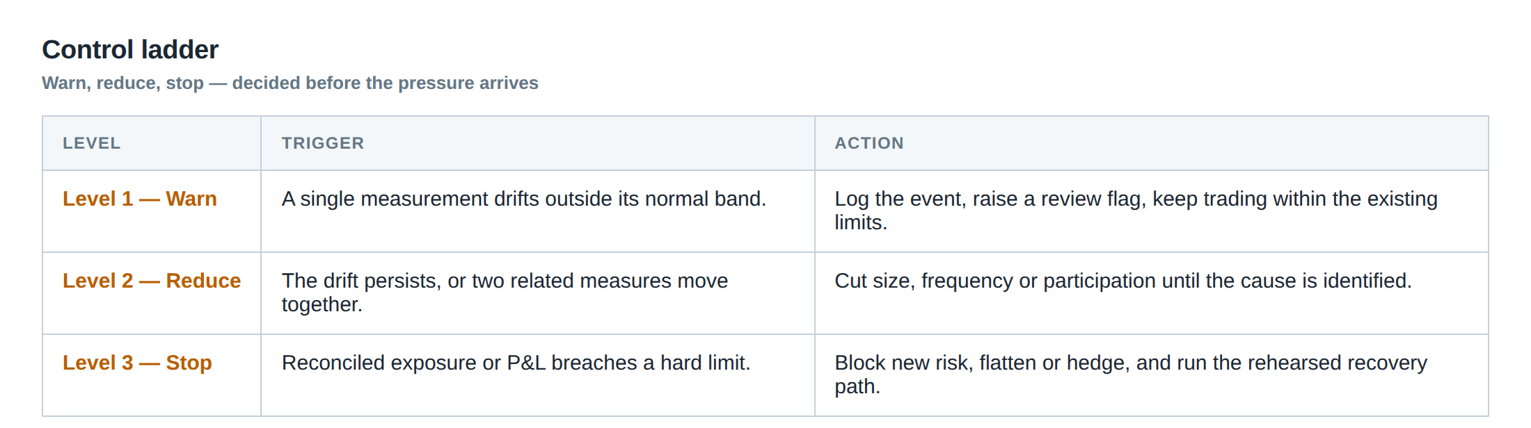
A layered defence is required. The first layer is a latency‑monitoring daemon that records the round‑trip time of every FIX message and raises an alarm when the 99th percentile exceeds a pre‑defined threshold, for example 120 ms for a sub‑second strategy. The second layer is a reject‑handler that treats any explicit exchange reject as a hard stop: the OMS immediately cancels all dependent child orders and flags the event for post‑mortem analysis.

The third layer is a partial‑fill guard. When a fill event reports less than 100 % of the requested quantity, the OMS checks the time elapsed since the order was sent. If the fill occurs after a latency outlier, the system automatically reduces the order size for subsequent attempts, thereby limiting exposure to the same adverse market condition.

The fourth layer is a stale‑data filter that compares the timestamp of the incoming market snapshot with a locally maintained clock. If the snapshot is older than a configurable horizon (e.g. 5 ms), the signal module is paused until a fresh snapshot arrives, preventing the generation of orders based on obsolete prices.

Finally, a fee‑impact estimator runs in parallel with the signal, recomputing the expected transaction cost whenever the cumulative daily volume crosses a fee tier. By adjusting the profitability threshold in real time, the system avoids entering trades that become marginal once the higher fee schedule applies.

How to measure whether it is working

The primary metric is the divergence between the research‑stage distribution of returns and the live‑stage distribution after applying all controls. One can compute the Kolmogorov–Smirnov statistic on the daily P&L series; a value below 0.05 indicates that the two distributions are statistically indistinguishable. Complementary to this, the tail‑risk measure – for example the 99.5 % Conditional Value‑at‑Risk (CVaR) – should not increase by more than a pre‑agreed factor, such as 1.2× the back‑tested CVaR.

Latency diagnostics provide a second set of gauges. The median latency should remain within the design envelope, but the key figure is the tail percentile: the 99.9 % latency must stay below the order‑cancellation deadline. A moving‑window plot of this percentile highlights periods of network stress that may require immediate remediation.

A third diagnostic is the fill‑ratio distribution. In the back‑test a fill ratio of 0.97 is assumed; live data should produce a distribution whose mean and variance match the simulated values within a tolerance band of ±0.02. Systematic deviations indicate either a mis‑calibrated market‑impact model or a hidden reject path.

By tracking these three families of metrics – distributional similarity, latency tail, and fill‑ratio fidelity – the desk can quantify the effectiveness of the production controls and trigger a review whenever the thresholds are breached.

The portfolio view

When production risk is managed at the stack level, the impact on the overall portfolio is measurable. The aggregate P&L curve smooths out individual order‑level anomalies, but the left‑hand tail of the portfolio return distribution is highly sensitive to rare latency spikes. A portfolio that appears robust in back‑test may exhibit a higher kurtosis in live trading if the control layer is insufficient.

Diversification across strategies with heterogeneous latency sensitivities can mitigate this effect. For instance, pairing a sub‑millisecond market‑making algorithm with a slower statistical‑arbitrage model reduces the probability that a single network outage will simultaneously affect both. However, diversification alone does not replace the need for per‑strategy production risk controls; the slow strategy may still suffer from stale‑data exposure that the fast strategy masks.

Risk‑adjusted performance metrics, such as the information ratio, should be recomputed using the live‑adjusted return series. If the information ratio drops by more than 10 % after accounting for production‑risk adjustments, the desk must revisit the execution design of the affected strategies. In practice, the portfolio manager monitors a dashboard that overlays the live‑adjusted Sharpe ratio with the latency‑tail metric, ensuring that any deterioration in one dimension is immediately visible in the other.

By treating production risk as an integral component of the risk model, rather than an after‑thought, the desk preserves the integrity of the portfolio’s risk‑return profile from the moment the back‑test ends to the moment the trade is settled.

—

Is your current execution stack capable of detecting and containing the latency‑tail events that turn a theoretically profitable signal into a loss in real time?

About the research behind this lesson

Andrew Lo's lectures build risk analysis from return distributions and statistical measures, rather than treating one realised result as a complete description of risk.

Applied to this lesson: For a fast strategy, median latency or average fill quality is not enough. The review has to include tail delays, stale-order frequency and the loss distribution when cancellation or routing behaves abnormally.

Explore PULSE: System details

PULSE live account: Verify the live account on FX Blue

Live chat and updates: Telegram @xtrskhft

Source: Risk and Return

Educational content only. Trading leveraged products involves risk.