October 26, 2026

⛶

What this problem really is

In a modern electronic market the most visible metric of a trading system is often the round‑trip latency – the time between a market data tick and the outbound order that attempts to capture the ensuing price move. The temptation is to equate every microsecond saved with a proportional increase in profit. In practice the relationship is far more nuanced. A strategy that can place an order five milliseconds earlier may still suffer a net loss if the order is rejected more often, if the realised spread after execution is eroded, or if the trade is entered only when the order book is already saturated with toxic flow. The core problem, therefore, is not speed in isolation but speed that translates into a better executable price, a higher probability of completion, or a lower exposure to adverse selection.

The market can be visualised as a series of price‑time‑priority queues. Each queue holds a mixture of genuine liquidity provision and hidden, often predatory, order flow. The value of a position in the queue is the sum of three components: the expected spread capture, the expected adverse‑selection cost, and the optionality of remaining in line for a future favourable move. When a trader measures only the elapsed time of an order, the optionality component is ignored, and the decision to keep the order alive becomes blind to the changing composition of the queue. Consequently, latency improvements that do not improve the balance of those three components are merely cosmetic.

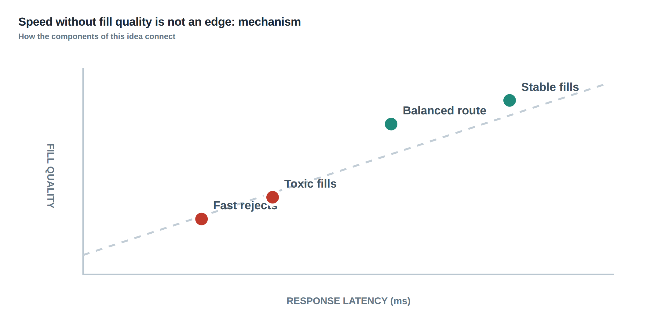
A robust edge therefore requires a holistic view that couples latency with fill quality metrics. The fill rate – the proportion of sent orders that result in a trade – must be examined alongside the realised spread – the difference between the execution price and the mid‑price at the moment of fill. Only when a faster decision consistently improves these two dimensions can the latency gain be considered a true edge.

How the mechanism works, step by step

The first step is the receipt of a market data update, typically a change in the best bid or ask. The data feed timestamps the event, and the order management system (OMS) evaluates whether the new price satisfies the strategy’s entry criteria. If it does, the OMS constructs an order packet, attaches a timestamp, and forwards it to the gateway.

At the gateway the packet is serialised, encrypted if required, and transmitted to the exchange’s matching engine. The exchange places the order at the back of the appropriate price‑time queue, where it co‑exists with other participants’ orders. While the order is waiting, the matching engine continuously matches incoming market orders against the queue, potentially moving the order forward or causing it to be cancelled automatically if the queue is depleted.

When a market order arrives that matches the price of the queued order, the engine executes a trade. The execution price is recorded, the trade is reported back to the OMS, and the OMS updates its internal position and risk tables. If instead the order is rejected – for example because the price moved out of the order’s limit, because the order exceeded the exchange’s size limits, or because the exchange applied a risk‑based throttling rule – the OMS receives a rejection notice. The distinction between a genuine execution and a fast rejection is crucial: a rejection consumes bandwidth, may increase the apparent latency of the system, and can inflate the measured fill rate if not filtered out.

Finally, the OMS must reassess the order’s place in the queue. If the market has moved unfavourably, the expected spread capture may have vanished, and the adverse‑selection risk may have risen. In such cases the system should cancel the order rather than let it sit idle, thereby preserving capital for more promising opportunities.

A worked example with real numbers

Consider a statistical arbitrage strategy that targets a 1.2‑tick spread on a liquid equity future. The baseline latency from market data receipt to order transmission is 30 ms, and the historical fill rate at that latency is 68 %. The realised spread on filled orders averages 0.95 ticks after accounting for slippage, giving a net edge of 0.25 ticks per trade.

The development team manages to shave five milliseconds from the pipeline, reducing the total latency to 25 ms. On paper this appears to be a 17 % improvement. However, the faster order now arrives at a point in the queue where the order book is already being consumed by aggressive market orders. The exchange’s risk engine flags the rapid influx of orders from the same source and doubles the automatic rejection rate from 12 % to 24 %. The fill rate consequently falls to 55 %.

More importantly, the orders that do get through tend to land when the order book is thin. The realised spread on those executions drops to 0.70 ticks, because the best opposite quote moves away within the extra five milliseconds that the order now spends waiting for a match. The net edge per trade is therefore reduced to 0.10 ticks, and the overall profit per hour collapses by roughly 60 % despite the latency gain.

If the strategy instead had introduced a pre‑trade filter that examined the depth of the book and the recent flow of market orders, it could have cancelled the order before it entered a toxic queue. By doing so, the rejection rate would have remained at 12 %, the fill rate would have stayed near 68 %, and the realised spread would have been preserved at 0.95 ticks. In this scenario the five‑millisecond reduction would have translated into a modest but genuine increase in realised profit.

Where it breaks in live markets

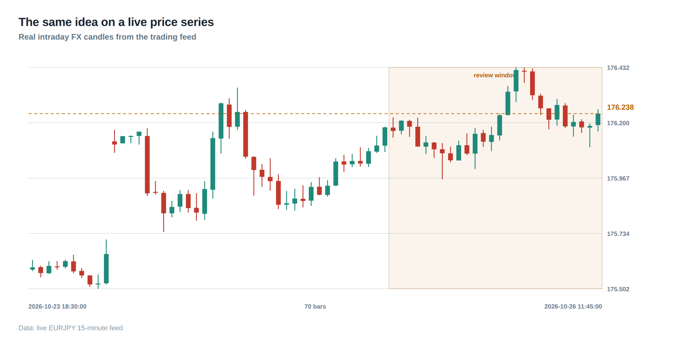
Live markets are rarely static; they oscillate between periods of calm liquidity and bursts of frantic, information‑driven trading. During high‑volatility regimes the order book depth can evaporate within a few milliseconds, and the probability that a newly placed order will be filled at the quoted price falls sharply. In such environments the option value of staying in line – the chance that the queue will move favourably – diminishes quickly, and the adverse‑selection cost rises.

Another common failure mode is the “toxic flow” scenario, where a large hidden order or a series of predatory market orders sweeps the best price levels as soon as they become available. A latency advantage that merely brings the order into the queue earlier does not protect it from being consumed by that flow; instead it may expose the order to a higher probability of execution at a worse price, or trigger a rejection if the exchange’s risk controls deem the order part of a potentially destabilising pattern.

Finally, many prop desks rely on a single latency metric – often the median round‑trip time – to gauge performance. This metric masks the distribution of outliers. A handful of unusually long latencies can cause a cascade of missed fills, while a large number of ultra‑fast rejections can inflate the apparent speed without delivering any executed volume. When the measurement framework ignores these outliers, the perceived edge becomes an illusion.

The operating path, stage by stage

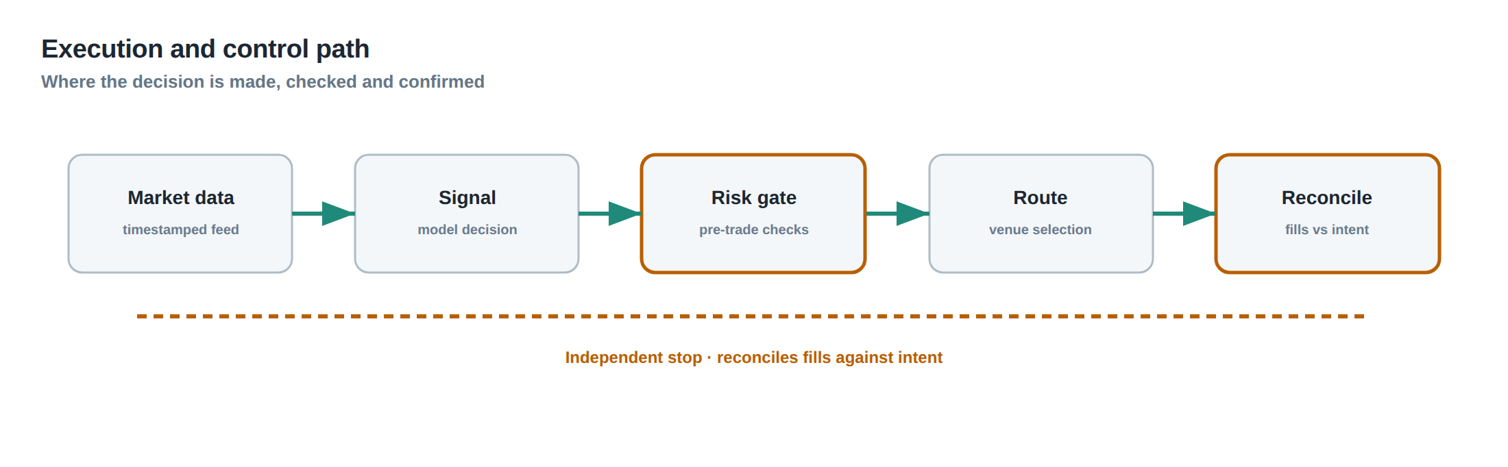
The first stage is data acquisition. Market data feeds are timestamped at the source, and the timestamps are synchronised across all feed handlers using a precision time protocol (PTP) or GPS‑disciplined clock. Any drift in this synchronisation directly contaminates the latency measurement and can lead to mis‑classification of fills versus rejections.

The second stage is decision logic. The OMS evaluates the incoming quote against the strategy’s statistical model, which incorporates not only price but also depth, order‑flow imbalance, and recent volatility. The decision must be made within a deterministic time budget; otherwise the latency budget is consumed before the order is even constructed.

The third stage is order construction and routing. Here the system adds the appropriate limit price, size, and any special instructions such as “post‑only” or “immediate‑or‑cancel”. The routing engine selects the venue based on a pre‑computed cost‑benefit matrix that includes expected fill probability, fee structure, and known latency to each exchange.

The fourth stage is exchange interaction. The order enters the price‑time queue, where its position is a function of the timestamp and the prevailing queue depth. The exchange may apply additional throttling or risk checks, which can result in a fast rejection that appears as a latency spike on the client side.

The final stage is post‑trade processing. The OMS records the execution price, updates the realised spread, and feeds the result back into the model for the next decision cycle. If the trade was rejected, the system must decide whether to retry, adjust the limit price, or abandon the opportunity altogether.

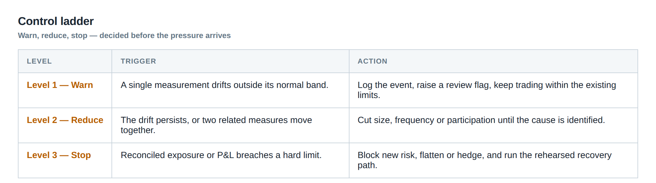
Controls that act before the damage

A layered defence is essential to prevent latency improvements from becoming detrimental. The first layer is a pre‑trade liquidity filter that examines the depth at the target price and the recent rate of change in the best bid/ask. If the depth falls below a configurable threshold, the order is either reduced in size or cancelled outright.

The second layer is a flow‑toxicity detector. By monitoring the sequence of market orders that hit the same price level, the system can infer the presence of a hidden aggressive participant. When the detector flags a high‑toxicity state, the OMS either switches to a more passive order type or postpones the trade until the flow normalises.

The third layer is a dynamic order‑lifetime manager. Rather than using a static timeout – for example “cancel after 50 ms” – the manager recalculates the expected value of remaining in the queue on each market data tick. If the expected spread capture falls below the adverse‑selection cost plus the option value of staying, the order is withdrawn before the timeout expires.

The fourth layer is a rejection‑rate monitor. It tracks the proportion of orders that are rejected within the first ten milliseconds after submission. A sudden rise triggers an automatic throttling of order flow to the affected venue, allowing the risk engine to stabilise and preventing a flood of useless rejections that would otherwise inflate latency statistics.

These controls work in concert to ensure that any latency gain is only realised when the underlying queue conditions are favourable. They also provide early warning signals that the market environment has shifted, prompting the strategy to adapt its parameters or to temporarily suspend activity.

How to measure whether it is working

Measurement must be multidimensional. The primary latency metric remains the median round‑trip time, but it must be reported alongside the fill‑rate curve – the proportion of orders filled as a function of elapsed time in the queue. A useful visualisation is a heat map that plots realised spread on the vertical axis and latency on the horizontal axis, with colour intensity representing fill probability.

Secondly, the rejection‑rate distribution should be split into “fast rejections” (those returned within 5 ms) and “slow rejections” (those that linger before being declined). Fast rejections often indicate that the exchange’s risk filters have acted, while slow rejections may point to network congestion or gateway overload.

Thirdly, the adverse‑selection cost must be estimated by comparing the execution price to the subsequent mid‑price movement over a short horizon, for example 100 ms. The average price drift after a fill provides a direct measure of how toxic the flow was at the moment of execution.

Finally, the overall profit‑and‑loss impact of the latency change should be assessed on a per‑venue basis, broken down by session (pre‑open, regular, after‑hours) and by volatility regime (low, medium, high). Only when the net contribution to the portfolio’s Sharpe ratio is positive can the latency improvement be declared successful.

The portfolio view

From a portfolio perspective the edge derived from speed is only a component of the total return stream. The realised spread, fill probability, and adverse‑selection cost together determine the expected profit per trade, which is then scaled by the number of opportunities the strategy can capture within a given time window. If a latency tweak reduces the expected profit per trade but allows the strategy to participate in a greater number of events, the net effect may still be favourable – but only if the increase in event count outweighs the loss in per‑trade quality.

Risk metrics such as maximum drawdown, value‑at‑risk, and turnover must be examined after the latency change. A higher turnover driven by more frequent, lower‑quality fills can inflate transaction costs and increase market impact, eroding the apparent edge. Moreover, the correlation structure of the strategy’s returns may shift if the latency improvement causes the algorithm to operate in a different slice of the order‑book dynamics. Portfolio managers therefore need to re‑optimise capital allocation, position sizing, and risk limits whenever a latency‑related parameter is altered.

In practice, the portfolio team will run a rolling back‑test that incorporates the new latency profile, the updated fill‑rate and spread statistics, and the revised rejection‑rate curve. The back‑test should be long enough to capture multiple volatility regimes and include a realistic simulation of order‑book toxicity. Only after the back‑test confirms an improvement in risk‑adjusted return should the change be rolled out to production.

The overarching lesson is that speed without fill quality is a mirage. A disciplined, data‑driven approach that measures the full spectrum of execution outcomes will reveal whether a latency gain truly adds value or merely shaves milliseconds off a losing proposition.

Will your next latency optimisation be judged by the quality of the trades it enables, or by the speed of the rejections it generates?

About the research behind this lesson

The seminar frames electronic markets as price-time-priority queues. It separates queue value into spread capture versus adverse-selection cost and the option value of retaining a place in line.

Applied to this lesson: An order lifetime therefore cannot be based on elapsed time alone: the system must reassess whether its queue position, expected spread and adverse-selection risk still justify keeping the order alive.

Two live systems, one desk

PULSE-X — power-packed HFT: high-frequency momentum on XAUUSD and EURUSD. System details · Live account

NIC-X — ultra-low drawdown: displaced-print arbitrage for large capital. System details · Live account

Start now: leave your email and request a free trial — we will send the pricing, the connection route and the trial terms. Pricing

Live chat and updates: Telegram @xtrskhft

Source: High-Frequency Trading and Modern Market Microstructure

Educational content only. Trading leveraged products involves risk.