October 31, 2026

What this problem really is

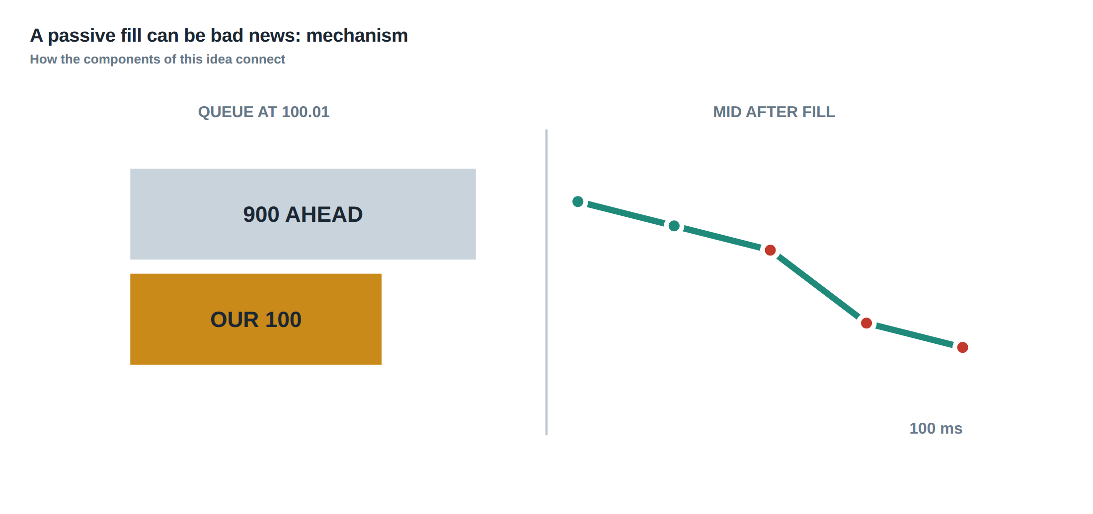
In electronic markets the most visible metric of an execution algorithm is its fill‑rate. A high percentage of orders that become trades is routinely celebrated as evidence of “good execution”. The reality is more nuanced. An order that is filled almost immediately after being sent may appear to be a perfect capture of the quoted spread, yet the same order may be sitting at the very front of a queue that is about to be swept by a large adverse price move. In that situation the fill is “passive” – it occurs without the trader having to cross the spread – but it is also “toxic” because the price subsequently moves against the position, eroding the captured spread and potentially turning a small profit into a loss.

The core issue is that fill‑rate alone does not distinguish between genuine spread capture and accidental exposure to adverse selection. When a trader’s order is constantly replenished, the aggregate of many tiny spreads can be wiped out by a single fill that precedes a sizeable move. The problem therefore lies in treating the queue as a static line measured only in seconds, rather than as a dynamic construct whose value changes with incoming volume, order‑cancellation patterns, and market micro‑structure signals such as order‑book imbalance and volatility.

To assess whether a high fill‑rate is truly beneficial, one must look beyond the binary “filled / not filled” outcome and examine the price path that follows each execution. Only by quantifying realised spread and the subsequent mid‑price drift can a desk decide if the algorithm is adding value or simply providing a conduit for toxic flow.

How the mechanism works, step by step

First, the algorithm estimates the volume that will arrive ahead of its own order. This estimate can be derived from recent order‑book dynamics – for example, the rate of aggressive market orders on the same side, the depth of the best‑bid or best‑ask, and the observed cancellation intensity of competing limit orders. The estimate is not a static number; it is refreshed on a sub‑second basis, reflecting the fact that order flow can accelerate dramatically in the seconds before a news release or a scheduled liquidity event.

Second, the system monitors cancellation dynamics. When competing orders are withdrawn, the queue position improves, but the same cancellations may also be a leading indicator of an imminent price move. A surge in cancellations on the ask side, for instance, often precedes a downward pressure on the mid‑price. By tracking the ratio of cancellations to new limit‑order submissions, the algorithm can infer whether the queue is stabilising or becoming fragile.

Third, after each fill the algorithm records the mid‑price movement over a predefined horizon – typically 5, 10, 20, and 50 ticks. The realised spread is calculated as the difference between the execution price and the mid‑price at the horizon, not the quoted half‑spread at the moment of execution. This captures the true cost (or benefit) of the trade, including any adverse selection that unfolds after the fill.

Finally, the results are segmented by market‑state variables: order‑book imbalance (the relative size of bid versus ask depth), realised volatility (standard deviation of mid‑price changes over the last minute), and venue (different exchanges or dark pools have distinct cancellation and latency profiles). By stratifying the data, the desk can identify under which conditions passive fills become toxic and adjust the order‑lifetime logic accordingly.

A worked example with real numbers

Consider a market maker who posts a 0.5‑tick limit sell order at the best ask on a liquid equity. The quoted spread is 1 tick, so the quoted half‑spread is 0.5 tick. Over the course of a trading session the algorithm sends ten identical orders, each with a target lifetime of 2 seconds.

Nine of the ten orders are filled within 300 ms of submission, each at the quoted price of 100.00 p. The mid‑price at the moment of each fill is 99.75 p, so the quoted spread capture appears to be 0.25 p per trade (0.5 p half‑spread). The realised spread is measured 10 ticks after each fill. In eight of the nine cases the mid‑price moves only a few tenths of a tick, leaving a realised spread of roughly 0.22 p per trade. The aggregate realised profit from the nine fills is therefore 9 × 0.22 p ≈ 1.98 p.

The tenth order, however, is filled at 99.95 p just before a sudden sell‑side imbalance. Within the next 5 ticks the mid‑price drops to 99.30 p, a move of 0.65 p. The realised spread for this single fill is therefore –0.40 p (execution price above the new mid‑price). The loss from this toxic fill exceeds the total profit from the nine earlier fills, wiping the net result to –0.42 p for the batch.

In this scenario the fill‑rate is 100 % and the quoted spread capture looks respectable, yet the realised performance is negative because a single adverse‑selection event dominates the profit stream. The example illustrates why the algorithm must monitor post‑fill price drift and adjust order lifetimes dynamically rather than relying on a static time‑based expiry.

Where it breaks in live markets

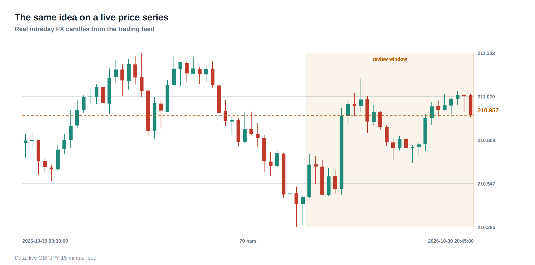
In live markets the assumptions that underpin a simple time‑based order‑lifetime model often collapse. During periods of heightened volatility – for instance, around macro‑economic announcements – the rate of aggressive market orders can surge by an order of magnitude. The queue that looked safe a few milliseconds earlier can be displaced within a single tick as liquidity evaporates.

Imbalance is another frequent breaking point. When the order‑book shows a strong skew – say, bid depth is 70 % of ask depth – the probability that a new sell limit order will be executed before the price moves down rises dramatically. The same imbalance that creates an attractive quoted spread also signals that the market is about to reprice, turning passive fills into toxic fills.

Venue‑specific quirks also matter. Some dark pools provide a “mid‑price” match but do not publish order‑book depth, making it difficult to estimate ahead‑of‑time volume. Latency differences between venues can cause an order to be filled on one exchange while a faster competitor on another venue already consumed the available liquidity, leaving the original order exposed to a price swing that it could not have anticipated.

These live‑market frictions mean that an algorithm that only tracks elapsed time will frequently keep orders alive long after their expected spread capture has evaporated, or will cancel them prematurely, missing out on genuine passive fills. The solution is to embed a continuous assessment of queue value that incorporates volume forecasts, cancellation signals, and post‑fill price dynamics.

The operating path, stage by stage

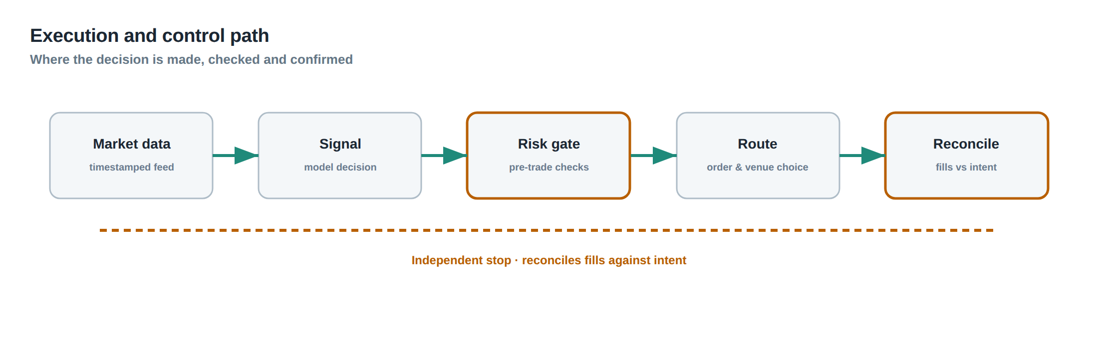
The first stage is market‑state ingestion. Real‑time snapshots of the limit‑order book are parsed to extract depth, imbalance, and recent cancellation counts. This raw data is fed into a short‑term volume‑ahead estimator, typically a weighted moving average of aggressive order flow on the same side of the book.

The second stage is queue‑valuation. Using the volume‑ahead estimate, the algorithm computes an expected “queue‑value” – the net of quoted spread capture, the probability of adverse selection, and the option value of remaining in line. The option value reflects the fact that staying in the queue gives the trader the right, but not the obligation, to capture the spread if the price does not move unfavourably.

The third stage is decision logic. If the queue‑value exceeds a pre‑set threshold, the order is left alive; if it falls below, the order is cancelled and possibly re‑submitted at a different price level or on a different venue. The threshold can be dynamic, scaling with realised volatility or with a risk budget allocated to adverse‑selection exposure.

The fourth stage is post‑fill analytics. Immediately after each execution, the system records the mid‑price at several horizons (e.g., 5, 10, 20 ticks) and updates a realised‑spread ledger. This ledger feeds back into the volume‑ahead estimator, allowing the model to learn which market‑state signatures tend to precede toxic fills.

The final stage is performance aggregation. Results are bucketed by imbalance band (e.g., –0.2 to –0.1, –0.1 to 0, 0 to 0.1, 0.1 to 0.2), volatility regime (low, medium, high), and venue. Within each bucket the algorithm computes average realised spread, fill‑rate, and the ratio of missed fills (orders that were cancelled before a favourable move) to toxic fills (fills that preceded an adverse move). This granular view informs the next iteration of the decision thresholds.

Controls that act before the damage

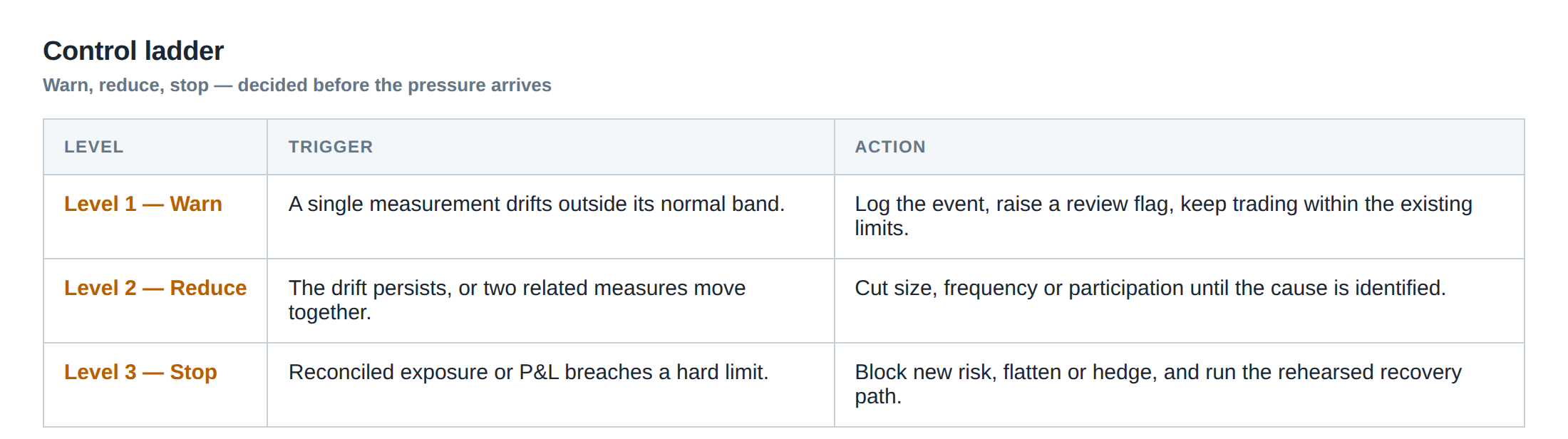
A robust control framework must intervene before a toxic fill can erode the profit stream. The first line of defence is a “pre‑fill filter” that evaluates the current imbalance and volatility. If the ask‑side depth is less than 30 % of bid‑side depth and the realised volatility over the past 30 seconds exceeds 0.8 ticks, the filter automatically tightens the order‑lifetime threshold, causing the order to be cancelled after 500 ms instead of the default 2 seconds.

The second control is a “cancellation‑rate monitor”. When the rate of order cancellations on the same side of the book spikes above a calibrated percentile (for example, the 90th percentile of the last hour), the system interprets this as a warning of impending price pressure and shortens the remaining lifetime of any standing orders.

The third control is a “venue‑switch guard”. If the realised spread on a primary exchange falls below a negative threshold for three consecutive fills, the algorithm temporarily redirects new orders to an alternative venue with a historically lower adverse‑selection profile under similar market conditions.

Finally, a “post‑fill loss‑stop” watches the realised spread of each fill. Should a fill generate a realised spread worse than –0.5 p within the first 5 ticks, the algorithm instantly suspends further order submissions for a short cooling period (e.g., 30 seconds) to avoid a cascade of toxic fills. These controls act in concert to keep the queue‑value positive and to prevent a single adverse event from destroying accumulated small spreads.

How to measure whether it is working

Measurement begins with the realised‑spread metric. For each fill, compute the difference between the execution price and the mid‑price at the chosen horizon; aggregate these differences to obtain an average realised spread per bucket (imbalance, volatility, venue). Compare this average to the quoted half‑spread; a positive gap indicates genuine spread capture, a negative gap signals toxic execution.

Next, calculate the “toxic‑fill ratio”, defined as the number of fills whose realised spread is negative divided by the total number of fills. A decreasing toxic‑fill ratio over time demonstrates that the pre‑emptive controls are effective.

A complementary metric is the “missed‑fill opportunity cost”. For each cancelled order, record the subsequent mid‑price movement over the same horizon used for realised spread. If the price moves in the direction favourable to the cancelled order by more than one tick, assign a cost equal to that move. Summing these costs provides an estimate of profit foregone by being overly aggressive in cancellations.

The final composite score is the net realised spread (total realised spread from fills minus total missed‑fill opportunity cost). When this net figure is positive and stable across market regimes, the execution strategy can be deemed successful. Regular reporting of these metrics, broken down by the segmentation dimensions, enables the desk to spot degradation early and to recalibrate thresholds before performance deteriorates.

The portfolio view

From a portfolio perspective, the impact of toxic passive fills is amplified by the correlation of positions across instruments. A single adverse‑selection event in a heavily weighted equity can offset the modest gains from dozens of small spreads in less liquid stocks. Therefore, the desk should monitor the aggregate realised spread of the entire portfolio, not merely the average per‑instrument figure.

Risk limits must incorporate a “toxic‑exposure” component: the maximum allowable proportion of the portfolio’s realised P&L that can be attributed to fills with negative realised spread. If the portfolio breaches this limit, the system should automatically tighten the queue‑valuation thresholds across all instruments, even those that have not yet shown toxicity.

Furthermore, the portfolio manager should consider the interaction between the execution algorithm and the market‑making inventory model. An inventory that is already skewed long may be especially vulnerable to a toxic sell‑side fill; conversely, a balanced inventory can absorb a few adverse fills without material impact. Integrating inventory risk metrics with the queue‑valuation engine creates a unified decision surface that respects both execution quality and overall capital utilisation.

In practice, the desk will run daily back‑tests that replay the full order flow, applying the current control parameters and measuring the net realised spread, toxic‑fill ratio, and missed‑fill cost. By comparing these back‑tests against a baseline where only fill‑rate is optimised, the desk can quantify the incremental value of the more sophisticated approach. Over time, this evidence base justifies the additional computational and operational complexity required to protect the portfolio from the hidden danger of seemingly benign passive fills.

Do you think your current execution metrics are sufficiently sensitive to the hidden cost of toxic passive fills, or could a deeper queue‑valuation framework improve your desk’s realised P&L?

About the research behind this lesson

The seminar frames electronic markets as price-time-priority queues. It separates queue value into spread capture versus adverse-selection cost and the option value of retaining a place in line.

Applied to this lesson: An order lifetime therefore cannot be based on elapsed time alone: the system must reassess whether its queue position, expected spread and adverse-selection risk still justify keeping the order alive.

Two live systems, one desk

PULSE-X — power-packed HFT: high-frequency momentum on XAUUSD and EURUSD. System details · Live account

NIC-X — ultra-low drawdown: displaced-print arbitrage for large capital. System details · Live account

Start now: leave your email and request a free trial — we will send the pricing, the connection route and the trial terms. Pricing

Join the market discussion: Telegram @squawklive

Source: High-Frequency Trading and Modern Market Microstructure

Educational content only. Trading leveraged products involves risk.