
XCore HFT / Trading Lab
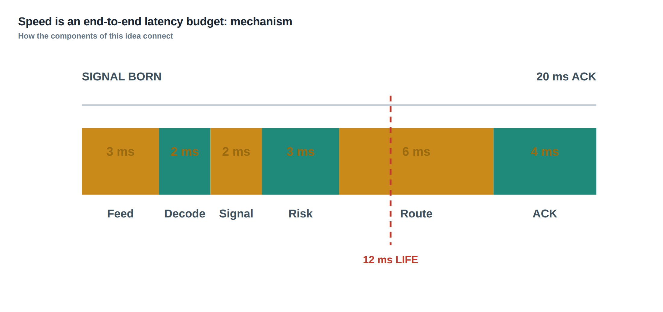
Speed is an end-to-end latency budget
Quantitative execution, market-microstructure, and risk-control research from XTRSK.
What this problem really is
The modern electronic market is a price‑time priority queue. Every incoming quote, every order, and every cancellation is placed in a line that moves forward only as time passes and as price improves. From the perspective of a prop‑trading desk the value of a strategy is the net of two forces: the ability to capture the spread and the cost of adverse selection incurred while waiting in the queue. Those two forces are not static; they evolve on a sub‑millisecond timescale. Consequently the “speed” of a strategy cannot be reduced to a single number such as “sub‑microsecond latency”. It is an end‑to‑end budget that must accommodate every useful stage from the instant the market data packet lands on the NIC to the moment the exchange acknowledges the execution. The slowest stage in that chain caps the effective half‑life of the signal, and if that half‑life is shorter than the total latency the signal will have decayed before the order can be acted upon. In practice the budget is a composite of feed transit, decoding, signal computation, risk checks, routing, and acknowledgement. Each component contributes to median latency, to the tail, and to jitter – the variability that makes worst‑case planning essential.
How the mechanism works, step by step
When a market data update arrives it first traverses the physical link between the exchange’s feed server and the trader’s data centre. The propagation delay is a function of distance and the medium (optical fibre versus microwave), typically measured in tens of microseconds for intra‑city links and up to a few hundred microseconds for cross‑continent routes. Once the packet reaches the NIC, the kernel or userspace driver must copy the payload into memory and hand it to the decoding engine. Modern kernels can achieve sub‑microsecond copy times, but any additional processing – checksum verification, packet re‑ordering, or loss recovery – adds jitter that is hard to predict.
The decoded tick is then fed to the pricing model. In a high‑frequency context the model may be a simple linear combination of order‑book imbalance, recent trade flow, and micro‑price dynamics. The computation itself is often bounded by memory bandwidth rather than raw CPU cycles; a two‑millisecond calculation is not unusual when the model incorporates several hundred symbols, each with multiple depth levels. After the raw signal is produced, the risk engine validates the order against position limits, credit exposure, and market‑specific constraints such as “no‑more‑than‑X% of the best‑price queue”. Only after passing these checks does the order get handed to the routing layer, which selects the appropriate gateway, builds the protocol‑specific message, and pushes it onto the outbound socket. The exchange’s gateway then acknowledges receipt, and finally the exchange’s matching engine either fills the order or rejects it. The total elapsed time from the first byte of market data to the acknowledgement is the end‑to‑end latency budget.
A worked example with real numbers
Consider a market‑making algorithm that monitors a liquid equity futures contract. The algorithm receives a depth‑5 snapshot every 100 µs. The feed travels over a 150 km microwave link, contributing roughly 0.5 ms of propagation delay. Decoding on a dual‑socket server adds 0.2 ms median, with a 99th‑percentile tail of 0.4 ms due to occasional packet re‑ordering. The signal computation, a weighted regression on the last 20 snapshots, takes 2 ms on the chosen CPU core. Risk checks, which involve a lookup of the current net‑position and a sanity check against a dynamic volatility band, consume 0.3 ms. Routing to the primary gateway, including packet construction and NIC transmission, adds another 0.6 ms, and the exchange’s acknowledgement latency averages 1.0 ms with a 95‑percentile of 1.5 ms.
Summing the medians yields a total of 4.6 ms, but the tail latency (median plus worst‑case contributions) stretches to about 5.5 ms. The signal’s half‑life – the time after which the predictive power of the current snapshot decays to 50 % – has been empirically measured at 12 ms for this instrument. If the order path were limited to 2 ms, the strategy would capture most of the spread. However, with the observed 20 ms complete path (including occasional network congestion spikes that push the routing latency to 3 ms and the acknowledgement to 2 ms), the order often reaches the exchange after the opportunity has already evaporated. In this scenario the two‑millisecond signal calculation adds little value; the dominant latency resides in the routing and acknowledgement stages, which together consume more than 80 % of the budget.
Where it breaks in live markets
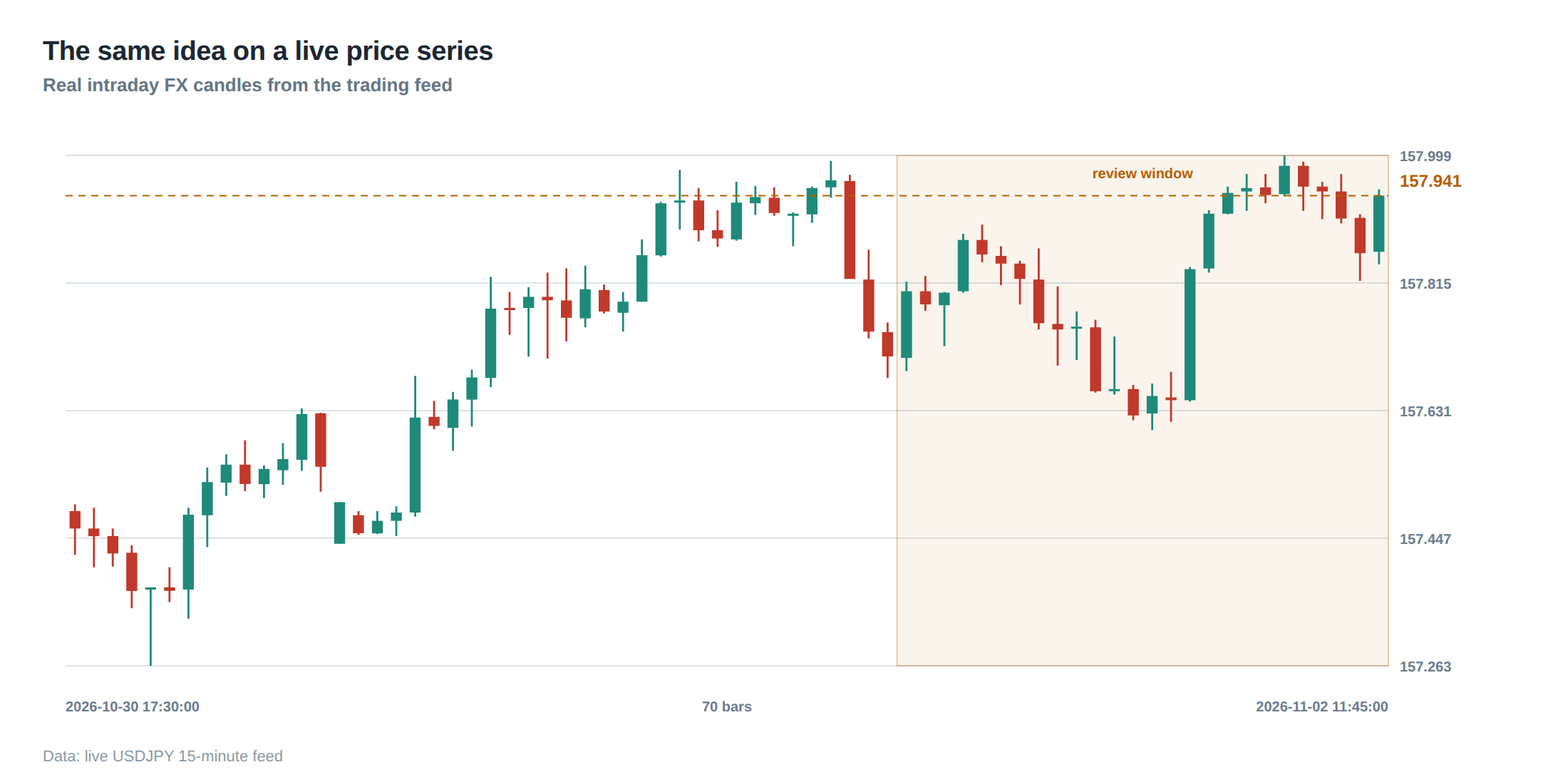
In live trading the idealised numbers above are perturbed by a host of externalities. Network congestion can cause packet loss, forcing the feed handler to request retransmission; each retransmission adds tens of microseconds of jitter that can push a previously acceptable tail into a catastrophic zone. Exchange‑side throttling, introduced to protect the order book from flood attacks, may delay acknowledgements when the order flow exceeds a hidden threshold. Moreover, the market microstructure itself is not static: during periods of heightened volatility the order‑book depth collapses, the spread widens, and the half‑life of any signal shrinks dramatically, sometimes to below 5 ms. In those moments the same end‑to‑end latency that was acceptable a minute earlier becomes a liability, causing the algorithm to post orders that are already stale, increasing adverse‑selection cost and eroding the spread capture.
Another failure mode is clock drift between the feed timestamp and the local system clock. If the timestamp attached to a market data packet is off by more than a few microseconds, the algorithm may mis‑align its internal state, treating a stale snapshot as fresh. The resulting signal will be mis‑priced, and the subsequent order may be placed at a price that no longer reflects the true market, again inflating the cost of adverse selection.
The operating path, stage by stage
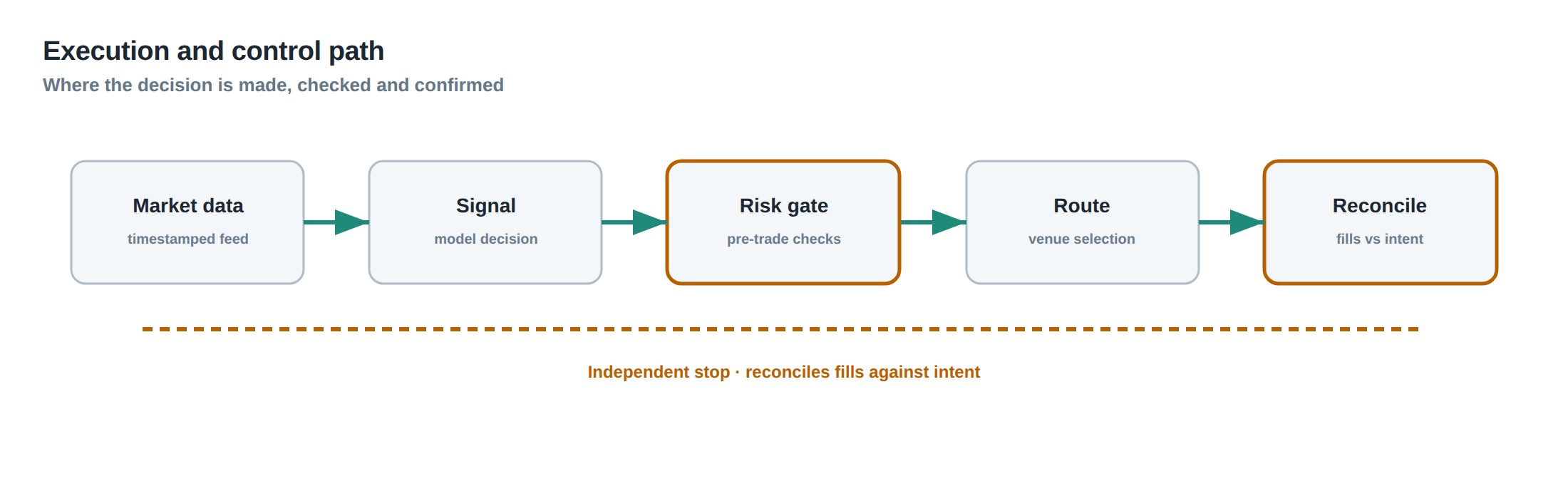
The end‑to‑end latency budget can be visualised as a cascade of stages, each with its own deterministic and stochastic components. First, the feed transit stage comprises physical propagation, encoding overhead at the exchange, and any intermediate aggregation points. Second, the decoding stage includes packet capture, checksum verification, and conversion from the exchange’s proprietary binary format to an in‑memory canonical representation. Third, the signal calculation stage is the heart of the algorithm, where statistical models ingest the decoded data and output a directional score. Fourth, the risk‑check stage validates the intended order against a matrix of limits that may be static (position caps) or dynamic (volatility‑adjusted exposure). Fifth, the routing stage selects the optimal gateway, constructs the order message in the exchange’s protocol, and hands it to the network stack. Finally, the acknowledgement stage measures the round‑trip time from the moment the order leaves the trader’s NIC until the exchange returns a fill or reject.
Each stage can be profiled independently, but the overall latency is not simply the sum of the medians; the tails interact. For example, a rare 1 ms spike in decoding can coincide with a 0.5 ms spike in routing, producing a 1.5 ms tail that would be invisible if each stage were examined in isolation. The operating path therefore demands a holistic view that records the timestamp at the entry and exit of every stage, using a common, synchronised clock source.
Controls that act before the damage
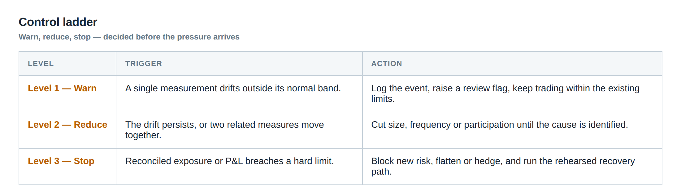
A robust latency management programme installs safeguards at the earliest possible point in the chain. The first line of defence is the feed‑handler configuration: selecting the fastest multicast group, enabling hardware timestamping on the NIC, and disabling any kernel‑level packet filtering that could introduce nondeterministic delays. At the decoding layer, lock‑free ring buffers and zero‑copy techniques keep the critical path short and eliminate memory‑copy jitter.
The signal engine can be throttled adaptively: if the measured end‑to‑end latency exceeds a pre‑defined fraction of the signal half‑life, the algorithm automatically de‑activates the most computationally intensive features, falling back to a lighter‑weight proxy that can produce a decision within a tighter window. Risk checks are similarly tiered; a fast pre‑check validates the most common limits, while a slower, more exhaustive check runs asynchronously and only blocks orders that would breach rare, high‑impact constraints.
Routing controls include pre‑established gateway health checks, automatic fail‑over to a secondary path when latency spikes, and the use of deterministic order‑routing tables that avoid runtime look‑ups. Finally, the acknowledgement stage benefits from exchange‑provided latency‑feedback channels that report the exact time the order entered the matching engine, allowing the trader to close the loop on clock synchronisation and to detect systematic delays that may arise from exchange‑side throttling.
How to measure whether it is working
Measurement must be continuous, granular, and anchored to a single time base. The preferred method is to embed hardware timestamps at the point of reception of the market data packet (using NIC‑level PTP or IEEE 1588) and at the moment the order packet leaves the NIC. The exchange’s acknowledgement packet also carries a timestamp generated by the matching engine; correlating the three timestamps yields the true end‑to‑end latency, free from software‑induced skew.
Statistical reporting should focus on median, 95th‑percentile, and 99.9th‑percentile latencies for each stage, as well as the jitter (standard deviation) of the total path. A useful diagnostic is the latency‑to‑half‑life ratio: if the median end‑to‑end latency exceeds 30 % of the signal half‑life, the strategy’s edge is likely being eroded. Tail latency is especially important; a 0.1 % tail that exceeds the half‑life can cause sporadic but costly mis‑executions that dominate the profit‑and‑loss over time.
Clock synchronisation quality must be audited daily. Drift beyond 1 µs between the feed timestamp and the local clock indicates a problem with the PTP grandmaster or with NIC timestamping, and should trigger an automatic alarm. The measurement system itself should be insulated from the trading stack: a dedicated monitoring server receives a mirrored copy of the data feed and the order flow, computes latency metrics, and publishes them to a read‑only dashboard, ensuring that the act of measurement does not perturb the latency budget.
The portfolio view
When latency is examined at the portfolio level, the interaction between multiple strategies becomes apparent. A latency‑intensive statistical arbitrage engine may consume a large share of the NIC’s processing cycles, inflating the jitter seen by a latency‑critical market‑making strategy that runs on the same server. Conversely, a fast market‑making algorithm that frequently sends small orders can saturate the exchange’s inbound gateway, provoking throttling that harms the slower strategy’s acknowledgement times.
Portfolio‑wide latency budgeting therefore requires allocating dedicated hardware resources – separate NICs, CPU cores, and even physical servers – to each latency‑sensitive class of strategy. Cross‑strategy risk checks must also be timed: a global position limit that is enforced after each order may become a bottleneck if the enforcement routine is serialised across strategies. By modelling the latency contribution of each strategy as a stochastic process and summing them, the desk can predict the probability that the combined tail exceeds the shortest signal half‑life in the portfolio, and can re‑balance resources accordingly.
In practice, the desk should maintain a latency heat‑map that records, for each instrument and each strategy, the median and tail latencies of every stage, the corresponding signal half‑life, and the realised profit‑per‑trade. Overlaying these maps reveals where latency is the limiting factor and where capital could be redeployed to higher‑return, lower‑latency opportunities.
—
If the slowest stage in your end‑to‑end chain is already longer than the half‑life of your most profitable signal, what concrete steps will you take to shrink that bottleneck?
About the research behind this lesson
The seminar frames electronic markets as price-time-priority queues. It separates queue value into spread capture versus adverse-selection cost and the option value of retaining a place in line.
Applied to this lesson: An order lifetime therefore cannot be based on elapsed time alone: the system must reassess whether its queue position, expected spread and adverse-selection risk still justify keeping the order alive.
Two live systems, one desk
PULSE-X — power-packed HFT: high-frequency momentum on XAUUSD and EURUSD. System details · Live account
NIC-X — ultra-low drawdown: displaced-print arbitrage for large capital. System details · Live account
Start now: leave your email and request a free trial — we will send the pricing, the connection route and the trial terms. Pricing
Join the market discussion: Telegram @squawklive
Source: High-Frequency Trading and Modern Market Microstructure
Educational content only. Trading leveraged products involves risk.
Chat with XTRSK
Chat ready
Start a chat and the XTRSK team will be notified immediately.