November 3, 2026

⛶

What this problem really is

The prevailing mantra on many prop desks is “the faster you are, the bigger the edge”. In practice the statement is incomplete because speed is only valuable when it translates into a better realised price, a higher probability of execution, or a lower risk of adverse selection. When a trader merely pushes an order five milliseconds earlier but the order is subsequently rejected, or only lands on the book during periods of toxic flow, the latency gain is a hollow statistic. The real problem is conflating raw response time with the economic quality of the resulting fill. An order that sits in the queue for ten micro‑seconds but captures the full quoted spread and survives the next price move is far more valuable than an order that is acknowledged in two micro‑seconds but is instantly cancelled by the market maker.

Electronic markets operate as price‑time‑priority queues. Each incoming limit order acquires a position in a line that is constantly reshaped by cancellations, market orders and new limit submissions. The value of that position is a combination of three components: the spread that can be captured if the order is filled, the adverse‑selection cost incurred when the market moves against the order, and the optionality of retaining the queue slot for a later, potentially more favourable move. When latency improvements are measured without reference to these components, the metric becomes a proxy for nothing more than the speed of the computer.

Consequently, any assessment of latency must be coupled with a measurement of fill quality. The two are inseparable: a faster decision that does not improve the realised spread, does not increase the fill rate, or worsens the post‑fill price trajectory does not constitute an edge. The desk must therefore treat latency as a means to an end, not an end in itself.

How the mechanism works, step by step

When a trading signal is generated, the order management system (OMS) timestamps the event and immediately decides on a venue, order type and price level. The order is then transmitted to the exchange gateway, where it enters the exchange’s matching engine. The engine assigns the order a queue position based on price and arrival time. At this stage the order’s “value” is the expected spread capture, which can be estimated from the mid‑price and the quoted bid‑ask.

While the order sits in the queue, two stochastic processes run in parallel. First, the market may move, narrowing or widening the spread, thereby altering the expected profit if the order is filled. Second, other participants may submit market orders or cancellations that shift the order’s position forward or backward, changing the probability of execution before the next price move. The OMS must continuously reassess whether the original decision remains optimal. If the expected spread has eroded or the adverse‑selection risk has risen above a pre‑defined threshold, the system may cancel or amend the order.

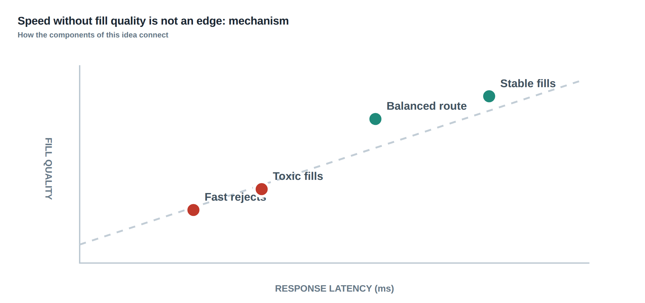
A crucial distinction appears at the moment of order acknowledgement. Some exchanges return a “rejection” almost instantaneously when the order would have been placed behind a large, hidden queue or when the venue’s risk controls deem the order unsafe. These fast rejections are not failures of latency; they are signals that the order would not have contributed positively to the queue. Conversely, a genuine execution – even if it occurs a few milliseconds later – represents a realised contribution to the strategy’s P&L. The system must therefore log both outcomes separately and treat them differently in performance attribution.

A worked example with real numbers

Consider a short‑term scalping strategy that posts a passive limit order at the best bid on a liquid equity futures contract. The baseline latency from signal to order entry is 25 ms. The strategy historically achieves a fill rate of 12 % per signal, with an average realised spread of 0.8 ticks (≈ $0.025) and an average adverse‑price movement of 0.2 ticks over the next 200 ms. The net expected profit per signal is therefore 0.6 ticks, or $0.01875.

The development team invests in a new network route that reduces the signal‑to‑gateway transmission time by 5 ms, bringing total latency to 20 ms. After deployment, the raw latency metric improves as expected, but the observed performance changes as follows: the fill rate drops to 7 % because the order now arrives at a moment when the order book is already saturated with aggressive market orders; the number of fast rejections doubles from 3 % to 6 % of total signals; and the realised spread on the remaining fills shrinks to 0.5 ticks while the adverse‑price movement rises to 0.3 ticks. The net profit per signal falls to 0.2 ticks (≈ $0.00625).

Even though the system is five milliseconds faster, the economic outcome deteriorates because the faster arrival pushes the order into a more toxic slice of the order flow. The key numbers – fill rate falling from 12 % to 7 %, rejection rate rising from 3 % to 6 %, realised spread shrinking from 0.8 to 0.5 ticks, and adverse movement increasing from 0.2 to 0.3 ticks – demonstrate that latency alone is not an edge. The strategy only benefits from speed when the faster decision improves the probability of a quality fill and does not expose the order to heightened adverse selection.

Where it breaks in live markets

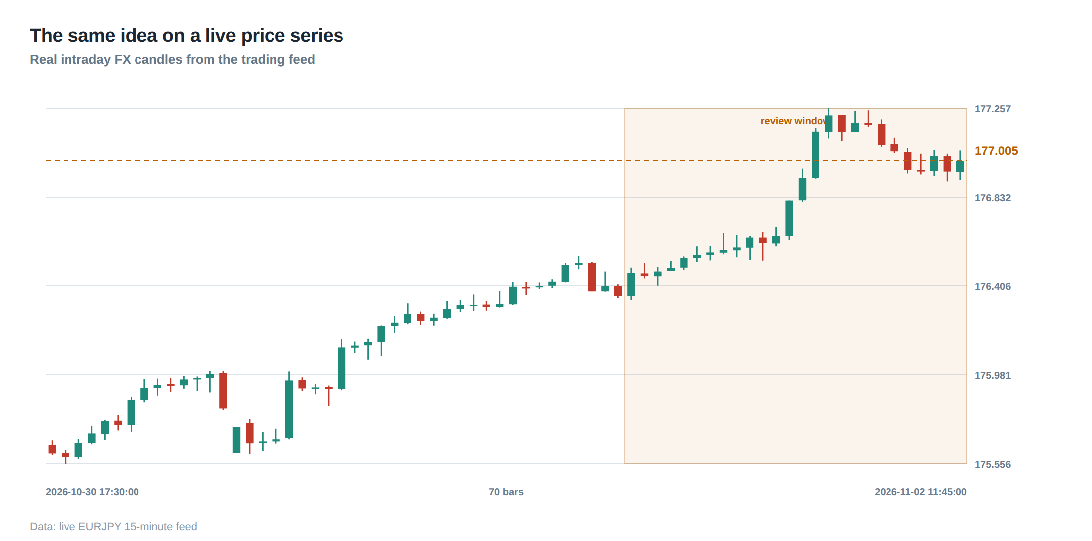
In live trading the idealised queue model is constantly perturbed by hidden liquidity, iceberg orders and dynamic maker‑taker rebates. During high‑volatility regimes, the order book depth can evaporate within a few milliseconds, turning a previously attractive price level into a trap. If a system continues to push orders based solely on latency, it may repeatedly chase a moving target, resulting in a surge of rejections and a spike in adverse‑selection losses.

Venue‑specific behaviours also create pitfalls. Some exchanges implement aggressive order‑cancellation penalties that increase the cost of frequent order churn, while others provide latency‑based priority boosts that only apply to orders that survive a minimum dwell time. Ignoring these nuances leads to a mismatch between the measured response time and the actual economic benefit. Moreover, session effects – such as the opening auction, lunchtime lull, or closing cross – alter the typical queue dynamics, meaning a latency improvement that is neutral at 10 am may be detrimental at 3 pm when the book is thin.

Finally, the presence of “toxic flow” – characterised by a high proportion of informed market orders – can render fast orders more likely to be filled just before a price move against the trader. In such environments, the marginal gain from shaving a few milliseconds is outweighed by the increased probability of being on the wrong side of the trade. The breakdown point is therefore a confluence of market microstructure, venue rules and volatility regime, not a simple latency threshold.

The operating path, stage by stage

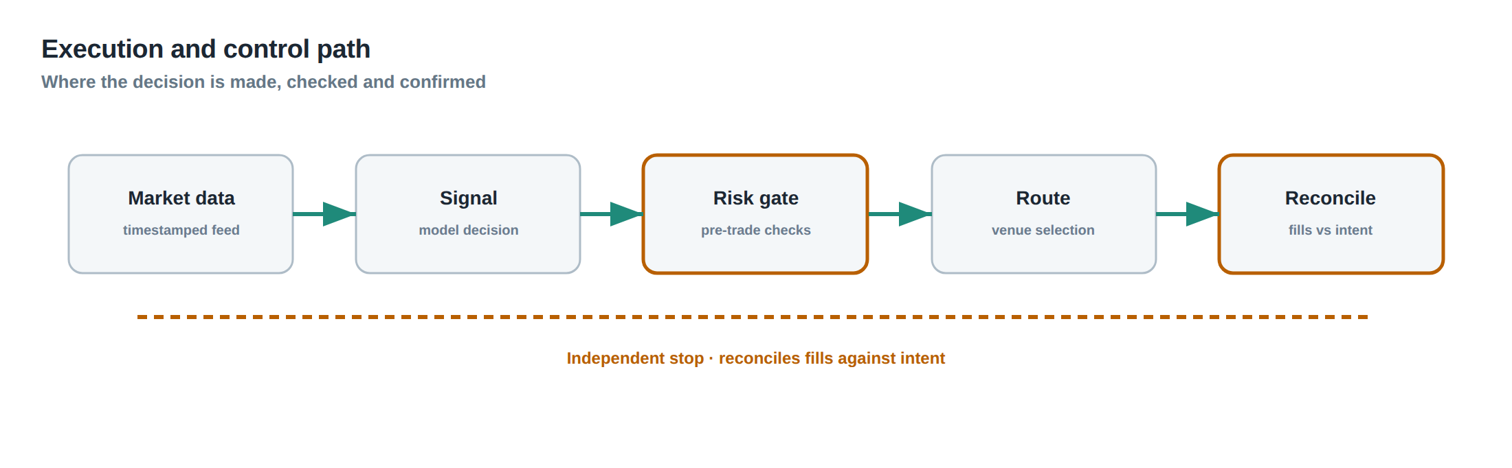
The first stage is signal generation, where the algorithm evaluates market data and produces a timestamped intent. The second stage is order construction, where the OMS selects venue, price, size and ancillary parameters such as post‑only or immediate‑or‑cancel flags. The third stage is transmission, encompassing network routing, protocol encoding and gateway processing. The fourth stage is exchange intake, where the order is placed into the matching engine’s queue and assigned a position. The fifth stage is execution monitoring, where the system records acknowledgements, fills, rejections and any subsequent price moves. The final stage is post‑trade analytics, where the realised spread, fill probability and adverse‑selection cost are calculated and fed back into the signal model.

At each stage, latency can be measured, but the decision to act on a faster measurement must be filtered through the expected economic impact. For example, a micro‑second gain in transmission (stage three) is only useful if the expected queue position improves enough to raise the fill probability by a measurable amount. If the same gain pushes the order into a queue already dominated by high‑frequency market makers, the net effect may be negative. Therefore, the operating path must embed conditional checks that compare the marginal latency benefit against the marginal change in expected profit.

Controls that act before the damage

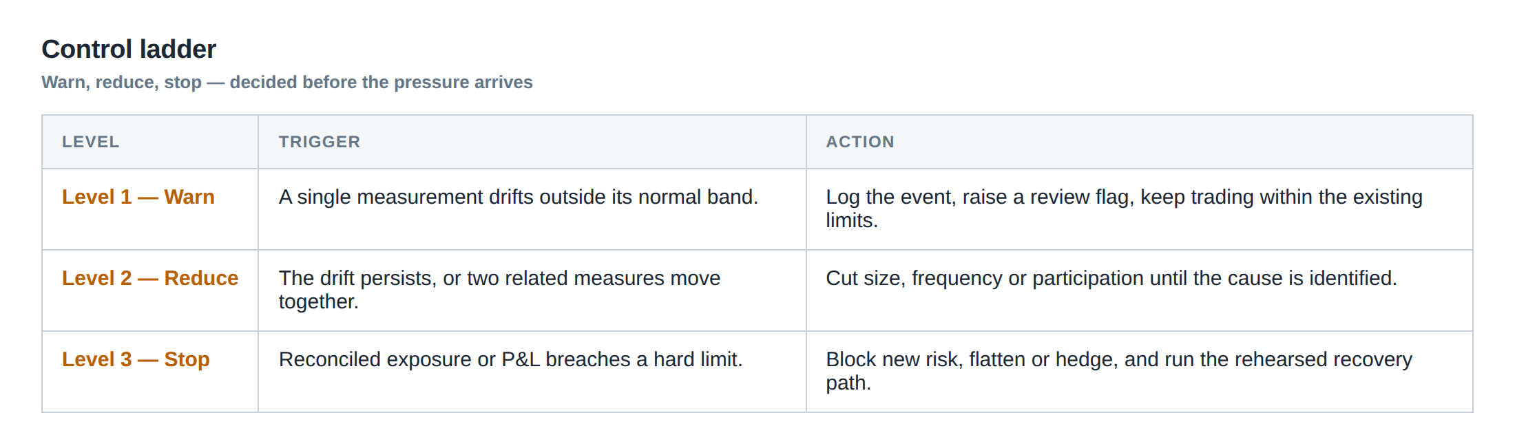
A robust control framework begins with a pre‑trade filter that evaluates the current order‑book state. If the depth at the target price is below a configurable threshold, the system either widens the price level or aborts the order, preventing placement in a thin, high‑risk slice. A second control monitors the rate of fast rejections; when the rejection frequency exceeds a set proportion of total attempts, the algorithm automatically backs off, reducing the order‑submission frequency or switching venues. A third layer assesses the realised spread over a rolling window; a sustained contraction signals that the market is no longer rewarding passive liquidity provision, prompting the strategy to switch to a more aggressive style.

These controls are implemented as state machines that can intervene before the order reaches the exchange, thereby avoiding wasted latency gains that would otherwise generate noise. They also maintain a feedback loop to the signal generator, allowing the model to adapt its aggressiveness based on recent micro‑structure conditions. By embedding these safeguards, the desk ensures that speed is exercised only when the surrounding environment validates the economic premise of the trade.

How to measure whether it is working

Measurement must go beyond simple latency statistics. The primary KPI is the realised spread per filled order, calculated as (execution price – mid‑price at the moment of fill) expressed in ticks. This should be paired with the fill rate, defined as the proportion of submitted orders that result in a genuine execution rather than a fast rejection. A secondary KPI is the adverse‑price movement, measured as the change in mid‑price over a fixed horizon (e.g., 200 ms) after the fill; the average of this metric quantifies the cost of adverse selection.

To isolate the effect of latency improvements, the desk should segment the data by venue, trading session and volatility regime. Within each segment, compare the pre‑ and post‑implementation values of the three KPIs. A statistically significant increase in realised spread or fill rate, coupled with a non‑significant rise in adverse‑price movement, indicates that the latency gain is delivering an economic edge. Conversely, if the fill rate falls or the adverse‑price movement rises, the latency improvement is likely detrimental.

Finally, the system should log the “queue‑value” at the moment of order entry – an estimate derived from the depth and order‑flow intensity – and track how this value evolves for orders that are later filled versus those that are rejected. Correlating queue‑value changes with latency adjustments provides a deeper diagnostic of whether speed is enhancing the underlying queue position or merely shifting the order into a less favourable part of the book.

The portfolio view

When the strategy is part of a broader portfolio, the marginal impact of latency on each individual instrument must be aggregated to assess the net effect on portfolio risk‑adjusted return. Faster fills on a high‑beta future may improve the Sharpe ratio, while the same speed on a low‑liquidity equity could increase turnover without adding profit, thereby inflating transaction costs. Portfolio‑level metrics such as total realised spread, aggregate fill rate and cumulative adverse‑selection loss should be monitored alongside traditional performance measures.

Moreover, latency‑related controls can be coordinated across strategies to avoid crowding. If multiple desks compete for the same queue position, a collective reduction in order‑submission aggressiveness during periods of high rejection rates can preserve overall market quality and reduce the likelihood of toxic flow. The portfolio manager should therefore treat latency optimisation as a shared resource, balancing the marginal benefit to each strategy against the systemic cost of increased order churn.

In practice, the desk should run periodic “edge‑validation” windows where latency is deliberately throttled to a baseline level, allowing a clean comparison of KPIs. If the portfolio’s net profit per trade declines when speed is restored, the desk has evidence that the latency gain is not an edge but a source of hidden cost. Conversely, a measurable uplift across the portfolio validates the investment in faster infrastructure.

Is the latency you are chasing truly delivering a better economic outcome, or merely shaving time from a process that already performs at its optimal point?

About the research behind this lesson

The seminar frames electronic markets as price-time-priority queues. It separates queue value into spread capture versus adverse-selection cost and the option value of retaining a place in line.

Applied to this lesson: An order lifetime therefore cannot be based on elapsed time alone: the system must reassess whether its queue position, expected spread and adverse-selection risk still justify keeping the order alive.

Two live systems, one desk

PULSE-X — power-packed HFT: high-frequency momentum on XAUUSD and EURUSD. System details · Live account

NIC-X — ultra-low drawdown: displaced-print arbitrage for large capital. System details · Live account

Start now: leave your email and request a free trial — we will send the pricing, the connection route and the trial terms. Pricing

Join the market discussion: Telegram @squawklive

Source: High-Frequency Trading and Modern Market Microstructure

Educational content only. Trading leveraged products involves risk.