November 5, 2026

What this problem really is

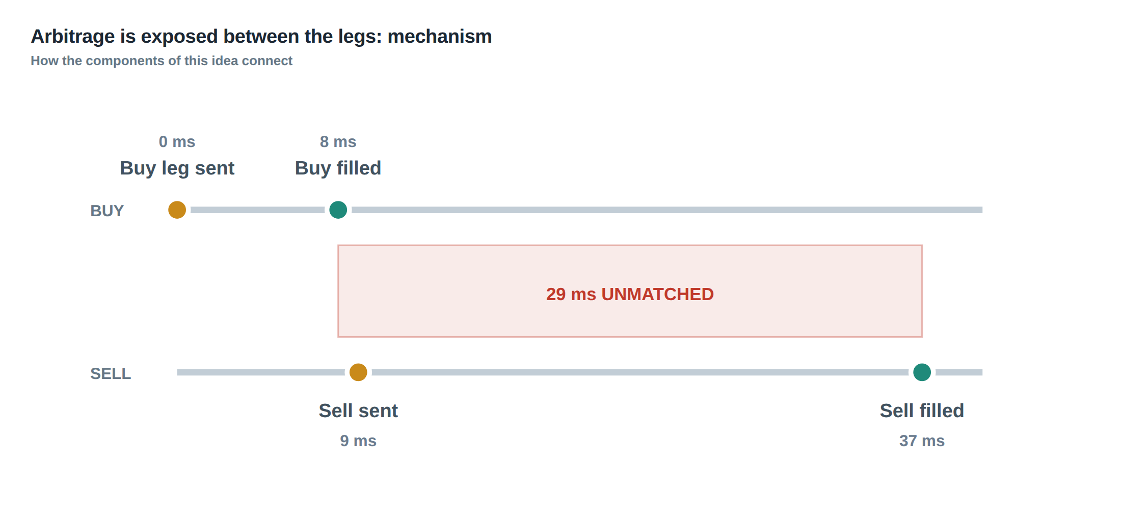
Arbitrage that appears in a spread is rarely a static, risk‑free construct. The moment a trader sends a buy order to one venue and a sell order to another, the two legs exist in different micro‑markets, each with its own queue dynamics, minimum‑size rules and latency profile. Until both legs are executed the position is not neutral; it carries a directional exposure that can be amplified by market moves, order‑book volatility or a sudden drop in liquidity. The core difficulty is that the “spread” is a conditional payoff – it materialises only if the two legs are filled within a pre‑defined window. If the window is breached, the trader is left with a net long or short that must be unwound, often at an adverse price.

The hidden risk is not merely the time lag but the information asymmetry that accrues while the order sits in the queue. In a price‑time‑priority system the order’s place in line is a valuable option: the longer it remains, the higher the probability of capturing the advertised spread, but also the higher the chance of adverse selection as the market moves away. Consequently, treating the spread as a static, market‑neutral bet is a mis‑characterisation; the exposure is dynamic and must be monitored after every market event.

A practical implication is that the trading system must keep a live ledger of filled versus remaining quantity for each leg, updating the risk profile after each partial fill, cancellation or amendment. Only by continuously reconciling the two sides can the desk decide whether the remaining exposure still qualifies as a “spread” or has morphed into a directional position that requires immediate hedging.

How the mechanism works, step by step

The first step is to decompose the intended arbitrage into its constituent legs and assign each a venue‑specific execution policy. For the buy leg the policy may be “post‑only, minimum 100 contracts, cancel if not filled within 150 ms”. For the sell leg the policy could be “marketable, minimum 50 contracts, reroute to an alternative venue after 80 ms of silence”. These policies translate into three quantitative thresholds: a hedge threshold (the point at which the net exposure exceeds a pre‑set risk limit), a cancel threshold (the maximum time or adverse‑price movement tolerated before pulling the order), and a reroute threshold (the condition under which the order is moved to a backup venue).

When the order is transmitted, the execution engine records the timestamp, the venue, the requested size and the minimum size constraint. As market data ticks arrive, the engine updates the filled‑quantity counter for each leg. If a partial fill occurs, the remaining quantity is recomputed and the expected completion‑time distribution is re‑estimated using recent fill‑rate statistics for that venue. This distribution is not static; it shifts with volatility, order‑book depth and the observed latency of the venue’s matching engine.

If the projected probability of completing the remaining quantity before the hedge threshold is breached falls below a configurable confidence level (for example 70 %), the engine triggers a mitigation action. The action can be a hedge order on a liquid reference market, a cancellation of the outstanding leg, or a reroute to a venue with a higher fill probability. The decision is made by weighing the expected spread capture against the adverse‑selection cost of staying in the queue, an approach that mirrors the option‑value reasoning of the underlying research.

A worked example with real numbers

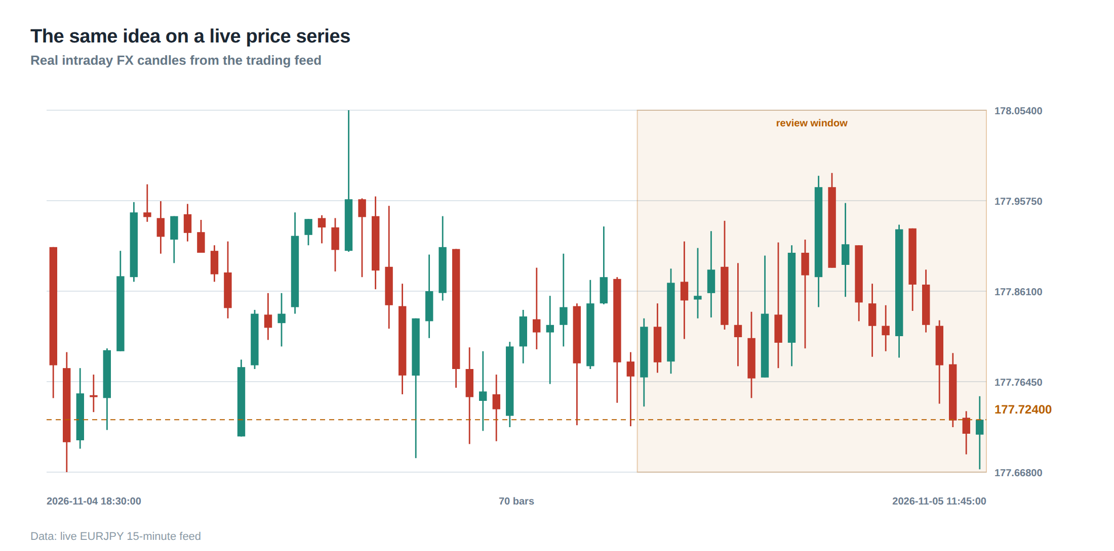
Consider a prop desk that spots a 5‑tick spread between two electronic futures markets. The buy leg is placed on Venue A at a limit price of 100.00 for 1 000 contracts, with a minimum order size of 100 contracts and a cancel‑after‑120 ms rule. Simultaneously a sell leg is posted on Venue B at a limit of 100.05 for the same 1 000 contracts, minimum size 50 contracts, and a reroute‑after‑90 ms rule. The expected fill rates, derived from the last hour of data, are 0.8 % per millisecond on Venue A and 0.6 % per millisecond on Venue B.

At t = 0 ms both orders are accepted into their respective queues. At t = 45 ms Venue A reports a partial fill of 300 contracts; the remaining buy quantity is now 700. At the same moment Venue B has not yet filled any contracts. The engine recomputes the completion‑time distribution: for the buy leg the median time to fill the remaining 700 contracts is 85 ms, while for the sell leg the median time to fill 1 000 contracts is 130 ms. Because the sell leg’s median exceeds the cancel‑after‑120 ms threshold, the system flags a potential breach of the hedge threshold.

At t = 95 ms the sell leg finally fills 200 contracts, leaving 800 contracts unfilled. The net exposure is now a long position of 800 contracts at an average cost of 100.00, with a short side of only 200 contracts at 100.05. The spread capture realised so far is (200 × 5 ticks) = 1 000 ticks, but the desk now carries a directional exposure of 800 contracts that must be neutralised. The engine evaluates the cost of hedging: buying a liquid index future at 100.02 incurs a 2‑tick slippage, while selling the same quantity on a third venue would cost 3 ticks due to lower depth. The optimal hedge is therefore a market order on the index future, costing 1 600 ticks (800 × 2). Adding the realised spread profit of 1 000 ticks yields a net loss of 600 ticks, illustrating how the interval between fills can turn an apparent arbitrage into a loss.

Where it breaks in live markets

In a live environment the assumptions that underpin the completion‑time distribution often collapse. Sudden order‑book imbalances, latency spikes, or a change in the venue’s minimum‑size rule can cause a leg to stall indefinitely. For example, a venue may raise its minimum execution size from 50 to 200 contracts during a volatility burst, instantly rendering a pending sell order invalid and forcing an immediate cancellation. The desk then faces a residual long that must be unwound in a market that may be moving against it.

Another common failure mode is the “queue‑jump” phenomenon, where a higher‑priority order is inserted ahead of the trader’s order due to a faster connection or a hidden order type. The expected spread capture drops, while the adverse‑selection risk rises because the market can move before the trader’s order reaches the front. If the system bases its lifetime decision solely on elapsed wall‑clock time, it will miss the fact that the queue position has deteriorated and that the probability of completing the leg within the hedge threshold has fallen dramatically.

Finally, cross‑venue latency asymmetry can create a hidden directional bias. If the buy leg is on a venue with sub‑millisecond latency and the sell leg on a venue with 200 ms average round‑trip, the buy side will tend to fill earlier, leaving the trader with a net long for a longer period. The longer that net exposure persists, the greater the chance that a market move will erode the spread. The system must therefore incorporate venue‑specific latency profiles into the real‑time risk assessment, not merely the aggregate time elapsed.

The operating path, stage by stage

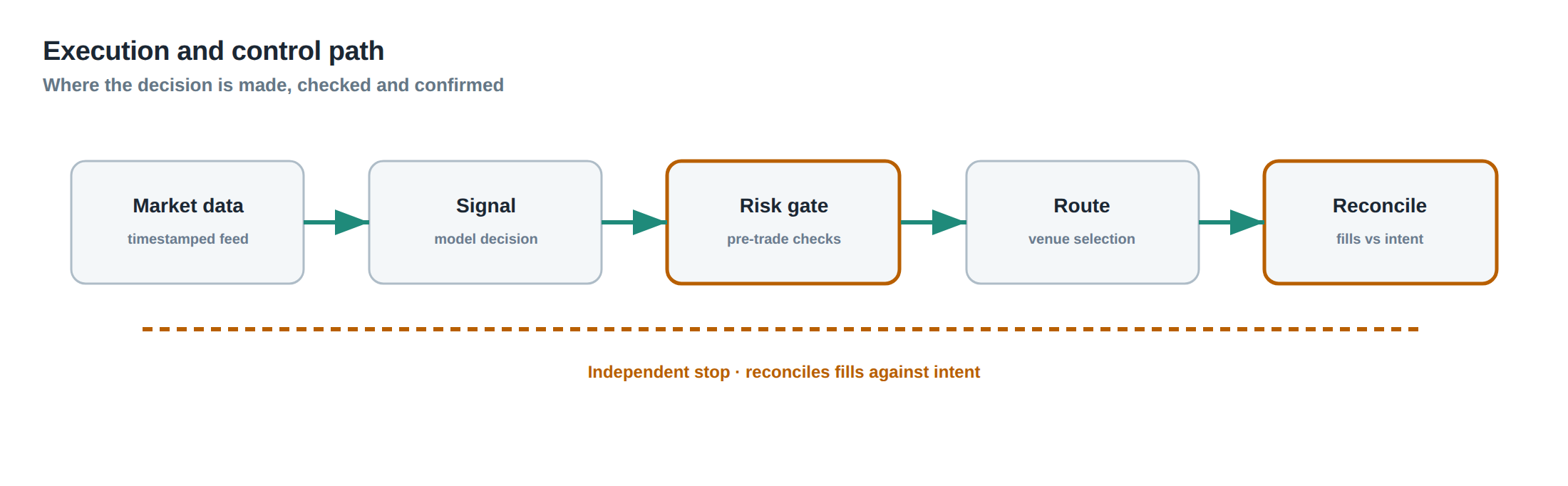
The first stage is order construction, where the trader specifies the target spread, the two venues, and the quantitative thresholds for hedge, cancel and reroute. The second stage is dispatch, during which the orders are sent to the matching engines and the engine records the initial timestamps and the minimum‑size constraints. The third stage is monitoring, where every market data event triggers an update of the filled‑quantity counters and a recomputation of the completion‑time distributions for the outstanding quantities. The fourth stage is decision, where the engine compares the projected probability of finishing both legs within the hedge window against the pre‑set confidence level; if the probability falls short, the engine selects the mitigation action with the highest expected utility. The fifth stage is execution of the mitigation – either placing a hedge order, cancelling the remaining leg, or rerouting it – and finally the sixth stage is post‑mortem analytics, where the realised spread, the cost of hedging, and the latency statistics are logged for performance attribution.

Each stage must be atomic and idempotent; a failure in one stage must not corrupt the state used in subsequent stages. The architecture therefore relies on a high‑throughput, low‑latency message bus that can deliver market‑data updates and order‑status events within microseconds, ensuring that the filled‑quantity ledger is always consistent with the external venues.

Controls that act before the damage

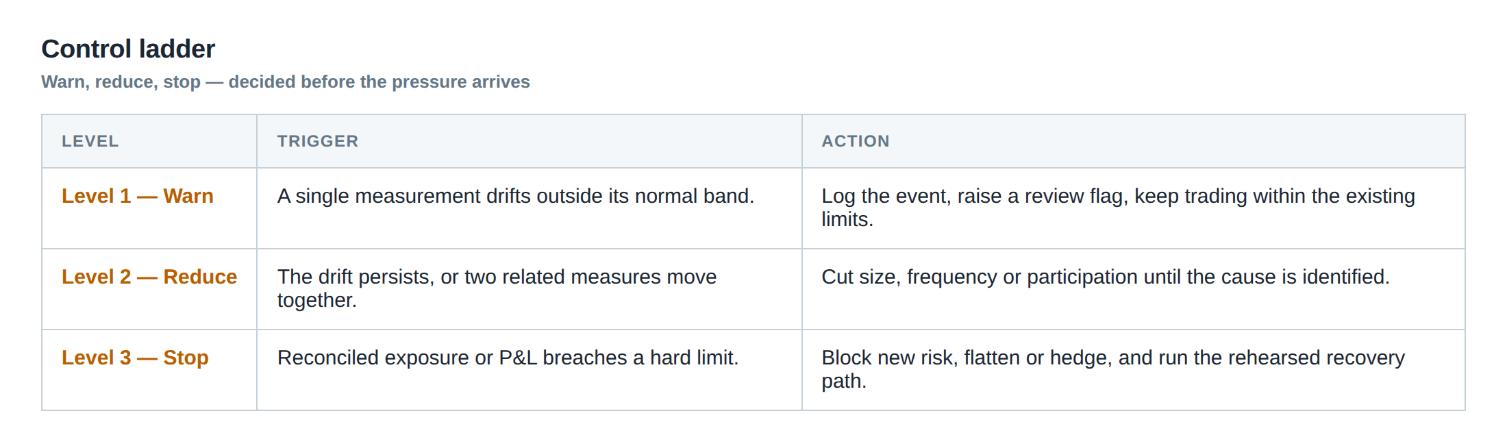
Preventive controls begin with static parameter checks: the minimum size of each leg must be compatible with the venue’s order‑book depth, and the aggregate size must respect the desk’s capital utilisation limits. Dynamic controls monitor the live fill‑rate against a moving benchmark; if the fill‑rate for a leg falls more than two standard deviations below its recent average, the system raises a “slow‑fill” flag. When the flag is active, the cancel‑after timer is accelerated, and the reroute threshold is lowered, prompting the engine to move the order to a more liquid venue before the hedge threshold is breached.

A further safeguard is the “pre‑emptive hedge” rule: if the net exposure after any partial fill exceeds a fraction (for example 30 %) of the total intended spread size, the system automatically sends a market‑neutralising hedge on a reference instrument, even if the opposite leg is still pending. This rule caps the directional risk that can accumulate while the spread is incomplete. Finally, a watchdog process audits the latency measurements of each venue every few seconds; any sudden increase beyond a defined envelope triggers a temporary suspension of new spread orders to that venue until the latency returns to normal.

How to measure whether it is working

Effectiveness is judged by three quantitative metrics. The first is the “completion ratio”, the proportion of spreads that achieve full fill of both legs within the hedge window. A healthy system typically maintains a ratio above 85 % in normal market conditions. The second metric is “net spread profit after hedge cost”, calculated as the realised spread capture minus the cost of any hedging or forced liquidation required to neutralise an unmatched leg. This figure should be positive on average, otherwise the spread strategy is bleeding. The third metric is “exposure time”, the average duration that a partial spread remains open before either completing or being mitigated; shorter exposure times indicate that the cancel and reroute thresholds are appropriately aggressive.

These metrics are collected per venue and per instrument, allowing the desk to spot systematic under‑performance. If a particular venue shows a consistently lower completion ratio, the parameters for that venue (minimum size, cancel timer) can be tightened. Likewise, an increase in exposure time may signal rising latency or a change in market microstructure that requires a revision of the hedge threshold.

The portfolio view

When spreads are executed across a basket of instruments, the individual leg risks aggregate into a portfolio‑level directional exposure. The desk therefore maintains a net‑position matrix that records the residual long or short for each instrument after each partial fill. By applying a correlation model to the instruments, the system can estimate the portfolio‑wide Value‑at‑Risk contributed by unfinished spreads. If the VaR contribution exceeds a pre‑defined limit, the system can automatically tighten the hedge thresholds across the board, or temporarily suspend new spread orders in the most correlated instruments.

Moreover, the profit‑and‑loss attribution must separate true spread capture from the P&L generated by hedging activity. This separation enables the desk to evaluate whether the spread strategy is adding alpha or merely providing a hedge for other directional bets. The portfolio view also informs capital allocation: venues that consistently deliver high completion ratios and low hedge costs can be allocated a larger notional budget, while under‑performing venues receive reduced exposure.

In practice, the portfolio‑level monitoring is run on a rolling window of 5 minutes, providing a near‑real‑time snapshot of the net directional risk. The desk can then make informed decisions about scaling the strategy up or down, adjusting thresholds, or reallocating capital to maintain a balanced risk‑return profile.

Is your current spread‑execution framework capable of detecting and mitigating the directional risk that accumulates between the fills of the two legs?

About the research behind this lesson

The seminar frames electronic markets as price-time-priority queues. It separates queue value into spread capture versus adverse-selection cost and the option value of retaining a place in line.

Applied to this lesson: An order lifetime therefore cannot be based on elapsed time alone: the system must reassess whether its queue position, expected spread and adverse-selection risk still justify keeping the order alive.

Two live systems, one desk

PULSE-X — power-packed HFT: high-frequency momentum on XAUUSD and EURUSD. System details · Live account

NIC-X — ultra-low drawdown: displaced-print arbitrage for large capital. System details · Live account

Start now: leave your email and request a free trial — we will send the pricing, the connection route and the trial terms. Pricing

Join the market discussion: Telegram @squawklive

Source: High-Frequency Trading and Modern Market Microstructure

Educational content only. Trading leveraged products involves risk.