November 6, 2026

What this problem really is

Statistical arbitrage is often presented as a low‑risk, high‑frequency profit engine built on the premise that two or more assets that have moved together in the past will continue to do so. In practice the premise is a model risk: the historical co‑movement is a statistical artefact that can evaporate the moment capital is deployed. When a trader opens a market‑neutral pair, the spread is assumed to be stationary, its mean‑reverting half‑life is estimated from a rolling window, and a z‑score threshold is used to trigger entry. The moment a sizeable order is placed, the market’s perception of the relationship can shift, liquidity can dry up, and the very act of trading can push the spread away from its historical mean. The result is a trade that appears arbitrage‑like on paper but behaves like a directional bet once the model’s assumptions are violated. The core thesis, therefore, is that historical co‑movement does not guarantee convergence after capital is committed; the risk lies not in the spread’s past but in the model’s ability to anticipate regime change, execution drag and funding constraints.

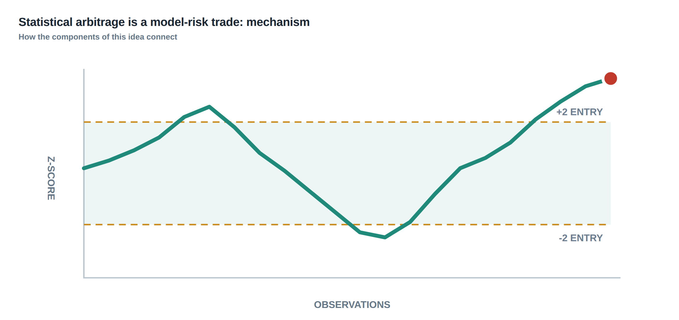
How the mechanism works, step by step

The first step is to identify a candidate spread, usually by regressing the price of one instrument on another and extracting the residual. The residual series is then tested for stationarity using Augmented Dickey‑Fuller or Phillips‑Perron tests across multiple market regimes – for example, a high‑volatility crisis period and a low‑volatility expansion period. If the null of a unit root is rejected in both regimes, the spread is deemed potentially mean‑reverting. The next step is to estimate the half‑life of reversion, typically by fitting an Ornstein‑Uhlenbeck process and solving \( \tau = \frac{\ln 2}{\kappa} \) where \( \kappa \) is the speed of mean reversion. The half‑life informs the expected holding period and therefore the exposure limit.

A second layer separates common‑factor exposure from the pure residual. Principal component analysis or a factor model isolates market, sector and macro‑factor betas; the residual after stripping these betas is the “pure spread” that the strategy aims to capture. This separation is crucial because a move in the common factor can generate a large apparent spread that is not a statistical arbitrage opportunity but a directional exposure.

Having isolated the residual, the strategy calculates a z‑score: \( z_t = \frac{r_t – \mu}{\sigma} \), where \( r_t \) is the current residual, \( \mu \) its long‑run mean and \( \sigma \) its standard deviation. When \( |z_t| \) exceeds a pre‑defined threshold, the model issues a signal. Before committing capital, the system adds a layer of cost adjustments: borrowing rates for short legs, funding rates for long legs, estimated turnover cost from the expected number of round‑trips per day, and slippage derived from recent order‑book depth. Only after the net expected profit exceeds a risk‑adjusted hurdle does the trade proceed.

Finally, the trade is bounded by both a price stop – a reversion threshold that, if breached, forces liquidation – and a time stop – a maximum holding period derived from the half‑life plus a safety buffer. If the spread fails to revert within the time stop, the position is closed regardless of the price, recognising that the underlying relationship may have altered.

A worked example with real numbers

Consider a pair consisting of Stock A and Stock B, both constituents of the same industry index. A linear regression over the past 250 trading days yields \( P_A = 1.12 P_B + \epsilon \) with an \( R^2 \) of 0.87. The residual series \( \epsilon_t \) passes the Augmented Dickey‑Fuller test at the 1 % level in both the 2008‑2009 crisis window and the 2016‑2019 expansion window, suggesting stationarity across regimes. Fitting an Ornstein‑Uhlenbeck process gives a mean‑reversion speed \( \kappa = 0.0045 \) per day, implying a half‑life of \( \tau = \frac{\ln 2}{0.0045} \approx 154 \) days.

The residual’s long‑run mean \( \mu \) is 0.03 % of the combined notional, and its standard deviation \( \sigma \) is 0.12 %. On the day of the signal the residual is 0.48 % above the mean, producing a z‑score of \( z = \frac{0.48-0.03}{0.12} = 3.75 \). The model’s price stop is set at a z‑score of 0.5, while the time stop is set at 1.5 × half‑life, i.e. 231 days.

Borrowing cost for the short leg of Stock B is 1.8 % annualised, funding cost for the long leg of Stock A is 0.9 % annualised. Expected turnover, based on an average of 1.2 round‑trips per day, translates to a transaction cost of 4 bps per trade. Slippage, measured from recent order‑book depth, adds another 2 bps. The gross expected convergence profit, assuming the residual reverts fully to the mean, is \( 0.48\% – 0.03\% = 0.45\% \) of notional. After subtracting borrowing (1.8 %/252 ≈ 0.007 % per day), funding (0.009 % per day), turnover (4 bps) and slippage (2 bps), the net expected profit per day is roughly 0.42 % – a favourable risk‑adjusted edge.

Because the z‑score is unusually high, the system inflates the position size variance to reflect the possibility of structural change or data error. Instead of allocating the full 2 % of the desk’s capital, the algorithm caps the exposure at 0.8 % of capital, reserving the remainder for other signals. The trade is entered with a market‑on‑close order for Stock A and a limit order for Stock B at a price that yields the target z‑score. The position is monitored hourly; if the residual moves back within a z‑score of 1.0, the exposure is scaled down proportionally. If after 180 days the residual remains above a z‑score of 0.8, the time stop triggers an exit, recognising that the historical relationship may have broken.

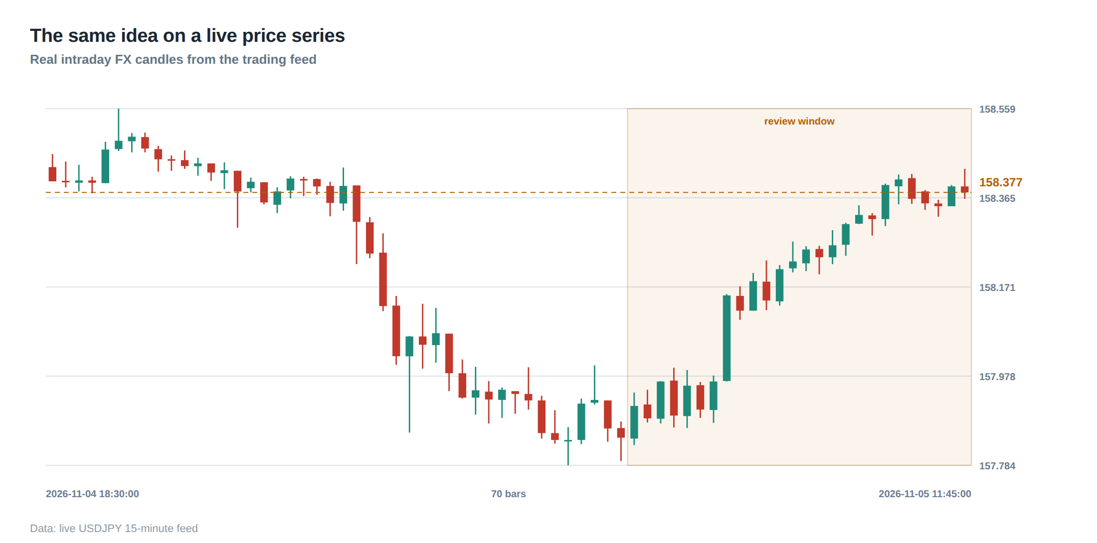
Where it breaks in live markets

In a live order‑driven market the spread is not a static number but a dynamic quantity that reacts to each new order. The moment a sizeable pair trade is placed, the order flow can compress the order book on one side and widen it on the other, creating a temporary widening of the spread that the model misinterprets as a larger arbitrage opportunity. Moreover, the queue‑value framework shows that the value of a limit order is the sum of expected spread capture, adverse‑selection cost and the option value of staying in line. If the queue position deteriorates because other participants jump ahead, the expected spread capture falls sharply, yet the order may still sit in the book, incurring financing costs without any realistic chance of execution.

Regime shifts compound the problem. A sudden change in volatility, a macro‑policy announcement, or a liquidity shock can alter the correlation structure that underpins the pair. The half‑life estimated from the previous regime becomes obsolete, and the residual may drift for weeks without reverting. In such circumstances a price stop alone is insufficient; the trade may sit at a favourable z‑score but accumulate funding and borrowing costs that erode the edge.

Data quality issues also surface. Missing quotes, delayed feeds, or corporate actions that have not been fully adjusted can produce spurious spikes in the residual, inflating the z‑score. A wide z‑score may therefore be a false signal, a harbinger of structural change, or simply a data glitch. Without robust validation, the algorithm can allocate excessive capital to a non‑existent opportunity, exposing the desk to unexpected losses.

The operating path, stage by stage

The first stage is data ingestion and sanitisation. Prices are aligned to a common timestamp, corporate actions are applied, and outlier filters flag any quote that deviates beyond three median absolute deviations from the rolling median. The second stage is model calibration: the regression coefficients, stationarity tests, and Ornstein‑Uhlenbeck parameters are recomputed on a rolling 250‑day window, with regime‑specific sub‑windows to capture divergent dynamics.

The third stage is signal generation. The residual is computed, the z‑score derived, and the price stop and time stop thresholds applied. If the z‑score exceeds the entry threshold, the system proceeds to cost assessment, adding borrow, funding, turnover and slippage estimates to the gross expected profit. Only when the net edge exceeds a pre‑set multiple of the portfolio’s volatility budget does the trade move to execution.

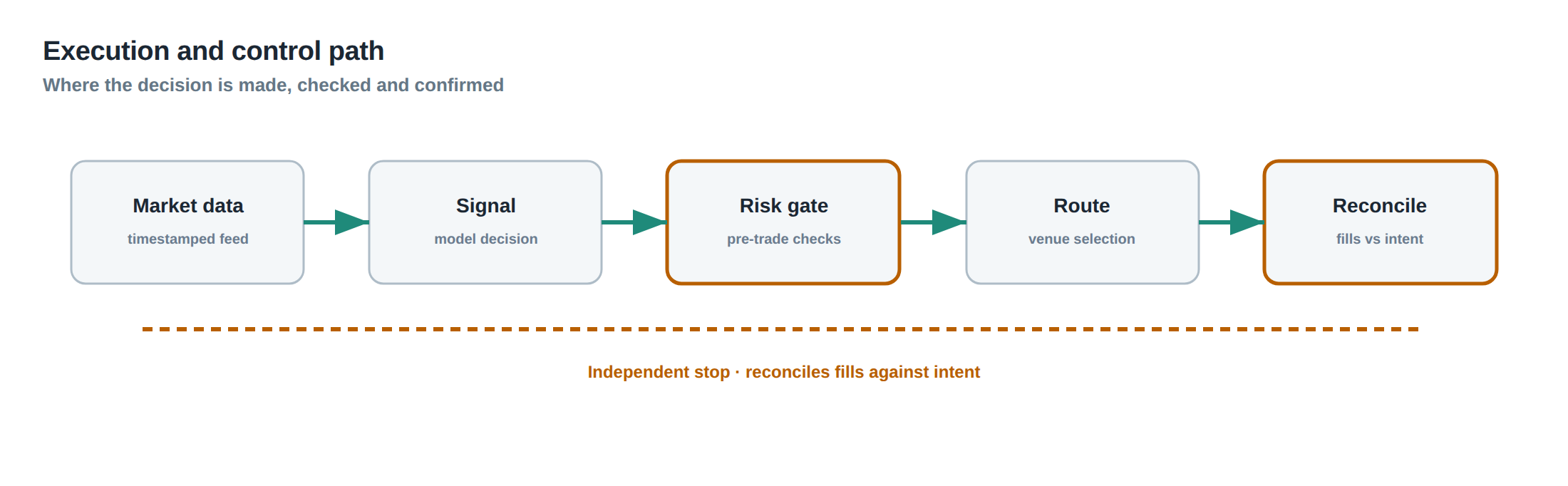
Execution is the fourth stage. Orders are routed to the venue offering the deepest queue for the required side, with a dynamic slice size that respects the desk’s turnover limit. The algorithm monitors queue position in real time; if the queue value falls below a minimum threshold, the order is cancelled and the trade is re‑evaluated.

The final stage is risk monitoring. The position’s exposure is capped at a percentage of capital that is automatically reduced if the residual’s half‑life lengthens beyond the original estimate. A time‑stop clock starts at entry; if the clock reaches the maximum holding period, the position is liquidated irrespective of price. Throughout, the system logs every decision point for post‑trade analysis.

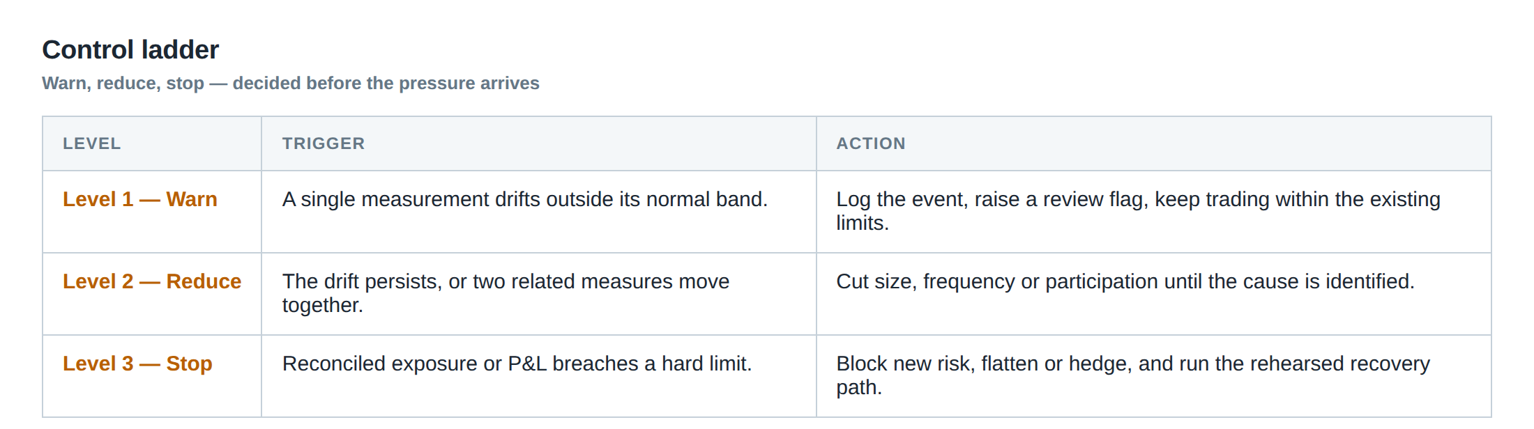
Controls that act before the damage

A ladder of pre‑trade controls guards against model breakdown. The first rung checks that the residual series passes stationarity tests in at least two recent regimes; failure aborts the signal. The second rung verifies that the estimated half‑life is less than twice the intended maximum holding period; a longer half‑life indicates a weak mean‑reversion signal and the trade is rejected.

The third rung isolates common‑factor exposure: the residual’s beta to the market, sector and macro factors must be below a pre‑defined threshold (typically 0.15). If the beta exceeds the limit, the trade is flagged for manual review because the spread may be contaminated by directional risk.

The fourth rung applies cost sanity checks. Borrowing rates are compared against the prevailing repo curve; if the short leg’s borrow cost exceeds the expected convergence profit by more than 30 %, the trade is discarded. Funding costs are similarly bounded.

The fifth rung enforces exposure caps that are dynamically adjusted when the relationship’s statistical metrics drift. If the rolling \( R^2 \) falls below 0.80 or the residual’s volatility spikes by more than 50 % relative to its 30‑day average, the maximum allowable notional is halved.

Finally, a real‑time queue‑value monitor evaluates the option value of staying in line. If the expected adverse‑selection cost rises above the spread capture estimate, the order is withdrawn before any capital is committed.

How to measure whether it is working

Performance is measured on two complementary axes: statistical fidelity and economic outcome. On the statistical side, the realised half‑life of each closed spread is compared with the pre‑trade estimate; a systematic upward bias indicates regime mis‑specification. The proportion of trades that close within the time stop versus those that breach the price stop provides a signal of model robustness.

Economically, the net realised P&L after all borrowing, funding, turnover and slippage costs is the primary metric. This figure is normalised by the realised capital at risk to obtain a risk‑adjusted return. A secondary metric is the “cost‑adjusted Sharpe”, where the denominator is the standard deviation of the net returns after deducting all explicit costs.

To capture model risk, the desk tracks the frequency of “wide‑z‑score” events that end in loss. If more than 20 % of such events result in a negative realised P&L, the threshold for position sizing is tightened. Stress‑testing on historical regime‑change periods (e.g., 2008‑2009, 2020‑2021) provides a forward‑looking estimate of tail loss.

Regular back‑testing with a walk‑forward window, combined with a Monte‑Carlo simulation that perturbs the residual’s drift and volatility, helps validate that the controls continue to filter out pathological cases.

The portfolio view

When the pair trade sits within a broader market‑neutral portfolio, its contribution must be evaluated in the context of overall factor exposure. The residual’s beta to the market, sector and macro factors is aggregated across all statistical‑arbitrage positions; the portfolio’s net exposure to each factor should remain within the desk’s risk budget.

Liquidity constraints are also portfolio‑wide. The sum of turnover from all pair trades is capped to avoid overwhelming the execution engine and to keep the average daily market impact below a predetermined threshold (often expressed in basis points of daily volume).

Funding and borrowing costs are pooled; the desk can offset a high borrowing rate on one short leg with a low funding rate on another long leg, reducing the net financing drag. However, the net cash‑flow profile must be monitored to avoid a funding shortfall that would force the desk to borrow at the unsecured rate, eroding the edge.

Finally, the portfolio’s risk‑adjusted return is compared against a benchmark that includes a synthetic statistical‑arbitrage index. If the desk’s contribution consistently underperforms the benchmark after costs, the underlying model assumptions are revisited, and the exposure caps are tightened or the pair universe is narrowed.

The overarching lesson is that statistical arbitrage is not a free‑lunch arbitrage but a model‑risk trade that demands continuous validation, cost discipline and dynamic exposure management.

Do you have a process in place to detect when a historically reliable spread has entered a new regime before capital is allocated?

About the research behind this lesson

The seminar frames electronic markets as price-time-priority queues. It separates queue value into spread capture versus adverse-selection cost and the option value of retaining a place in line.

Applied to this lesson: An order lifetime therefore cannot be based on elapsed time alone: the system must reassess whether its queue position, expected spread and adverse-selection risk still justify keeping the order alive.

Two live systems, one desk

PULSE-X — power-packed HFT: high-frequency momentum on XAUUSD and EURUSD. System details · Live account

NIC-X — ultra-low drawdown: displaced-print arbitrage for large capital. System details · Live account

Start now: leave your email and request a free trial — we will send the pricing, the connection route and the trial terms. Pricing

Join the market discussion: Telegram @squawklive

Source: High-Frequency Trading and Modern Market Microstructure

Educational content only. Trading leveraged products involves risk.