November 6, 2026

What this problem really is

Cross‑venue arbitrage is often presented as a simple “buy low, sell high” on two order books that appear to diverge by a few ticks. In practice the two displayed prices are only the tip of a deeper liquidity structure. The arbitrageur must be able to execute both legs at the displayed depth, settle the trades under the respective venue rules, and move the resulting inventory without incurring prohibitive costs or timing risk. If any of those components is blocked – for example because the settlement cycle on one exchange is T+2 while the other settles instantly, or because a withdrawal limit caps the amount that can be moved in the required window – the apparent price gap is not a real, executable arbitrage. The problem therefore lies not in the static quote gap but in the dynamic transferability of the resulting position across venues, after fees, rebates, funding costs and operational constraints have been applied.

How the mechanism works, step by step

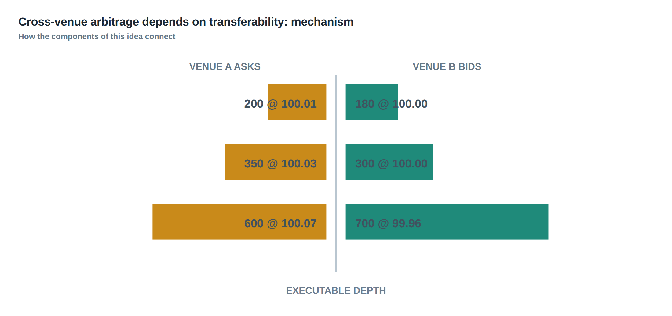
The first step is to query the depth of both venues. Rather than relying on the best‑bid/best‑ask, the algorithm extracts the cumulative volume at each price level until the desired trade size is covered. This “executable depth” determines the true price at which the leg can be filled. The second step adds the venue‑specific transaction costs: taker fees, maker rebates, clearing fees and any funding charges for margin accounts. The third step projects the settlement timeline – whether the trade settles on a gross‑net basis, requires a cash‑and‑carry, or is subject to a delayed cash‑out process. The fourth step evaluates the transfer pipeline: the speed at which the realised inventory can be moved, the limits on daily withdrawal, and any latency introduced by internal settlement systems. Only when the net proceeds after all adjustments exceed the cost of moving the inventory does the arbitrage become viable.

A worked example with real numbers

Consider a futures contract on a high‑liquidity index that trades on Exchange A and Exchange B. On Exchange A the best ask for 10 contracts is 4 250.00, with a taker fee of 0.02 % and a maker rebate of 0.01 % for any residual limit orders placed to unwind the position. On Exchange B the best bid for the same size is 4 255.00, but the venue imposes a taker fee of 0.03 % and a withdrawal limit of 5 contracts per minute. The raw spread is therefore 5.00 points.

Applying fees, the cost to buy on A is 4 250.00 × 10 × (1 + 0.0002) = 42 502.00. The proceeds from selling on B are 4 255.00 × 10 × (1 – 0.0003) = 42 517.85. The gross profit before transfer costs is 15.85 points, or 15.85 × $10 = $158.50 per contract (assuming a $10 multiplier).

Now incorporate the withdrawal constraint. Because only five contracts can be moved out of Exchange B each minute, the trader must either pre‑position five contracts on B or accept a half‑size arbitrage. If the trader decides to pre‑position, they must hold five contracts on B overnight, incurring a funding charge of 0.005 % per day. Over a 24‑hour holding period the funding cost is 4 255.00 × 5 × 0.00005 = $1.06.

Finally, add the latency risk. If the internal settlement system requires 30 seconds to credit the cash from Exchange A to the account that can withdraw from B, a sudden price move of 2 points on B would erode the net profit. In this scenario the net after‑cost profit is 15.85 – (0.02 + 0.03) = 15.80 points, minus $1.06 funding, leaving roughly $157.40. The arbitrage is still positive, but only because the trader pre‑positioned inventory and accepted the funding drag. If the pre‑position had not been in place, the withdrawal limit would have forced a partial fill, reducing the realised spread to 2.5 points and turning the trade marginally unprofitable after fees.

Where it breaks in live markets

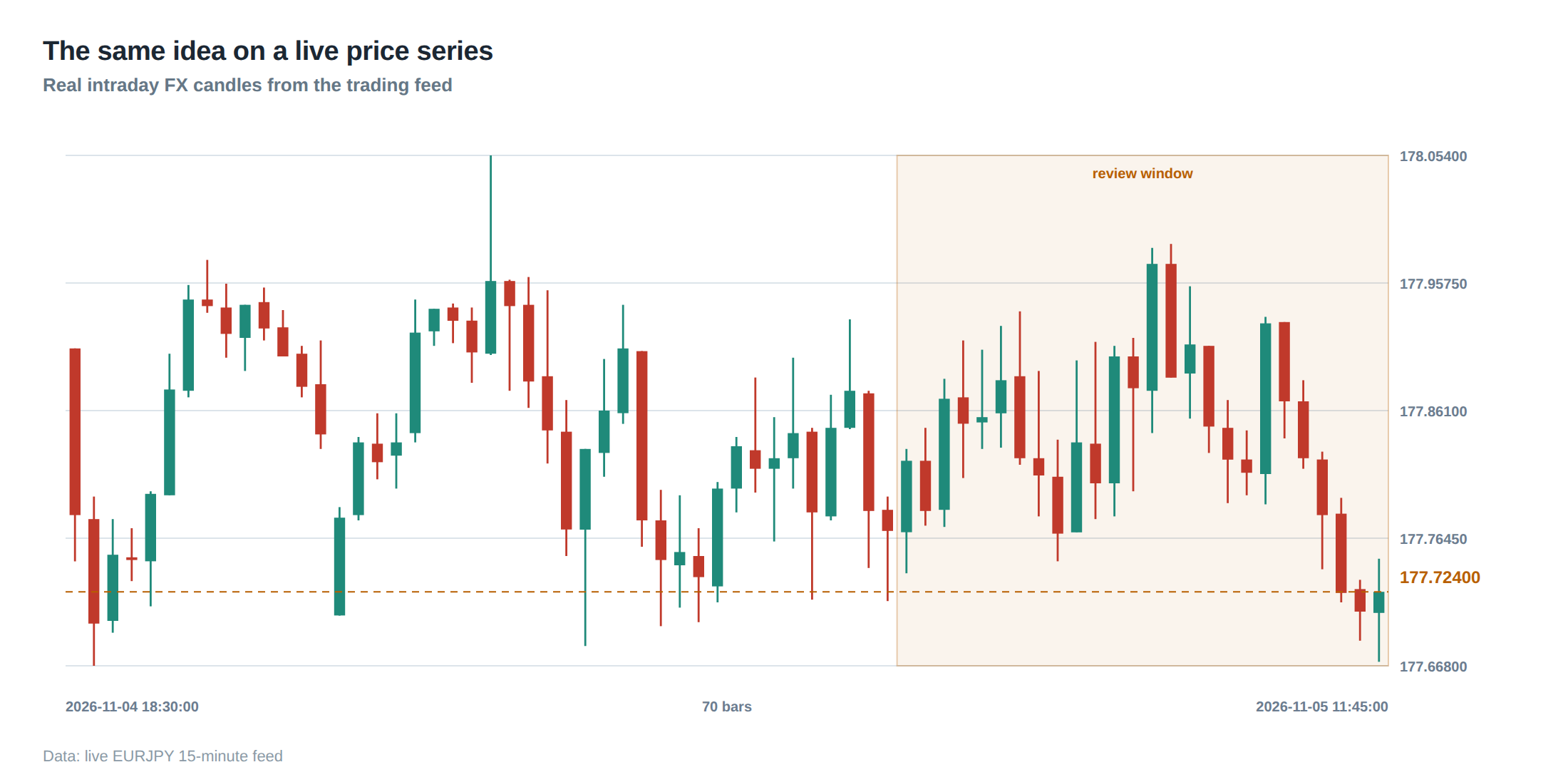
The theoretical profit collapses as soon as any of the transfer steps stalls. A venue outage – for instance a temporary disconnect of Exchange B’s API – prevents the sell order from reaching the market, leaving the bought inventory stranded on Exchange A where it may be subject to overnight financing. Counter‑party exposure also rises: if the clearing house of Exchange B requires a margin call before the position can be liquidated, the trader may be forced to post additional collateral, eroding the spread. Withdrawal caps, anti‑money‑laundering throttles, and cross‑border settlement delays are often hidden in the terms of service but become decisive when the arbitrage window is measured in seconds rather than minutes. Moreover, the presence of high‑frequency market makers can consume the displayed depth within milliseconds, turning a seemingly executable gap into a phantom.

The operating path, stage by stage

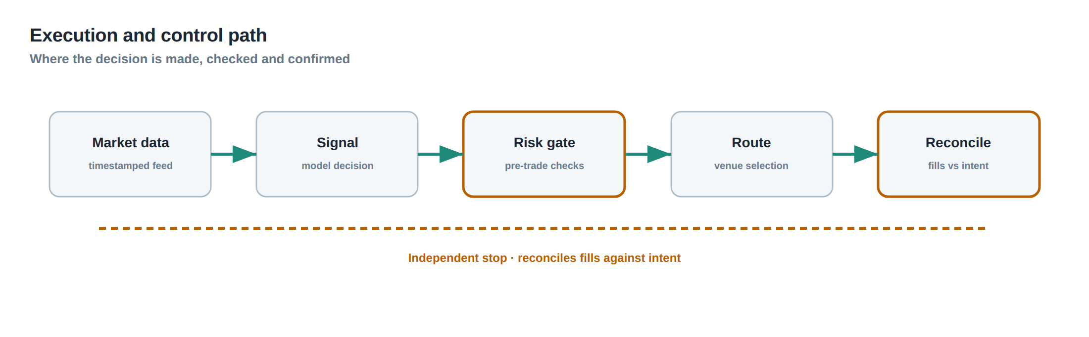
The operational workflow can be visualised as a linear chain of checks. First, the market‑data feed validates that the executable depth on both sides exceeds the intended size. Second, a cost‑model module overlays fees, rebates and funding to compute a net‑spread. Third, a transfer‑engine evaluates inventory location, withdrawal limits and expected latency, returning a binary “transfer‑feasible” flag. Fourth, a risk‑monitor interrogates the counter‑party credit limits and margin utilisation on each venue. Finally, the execution engine submits a paired order set – a taker order on the cheap side and a maker order on the expensive side – with a shared identifier to enable atomic cancellation if any leg fails to acknowledge within a pre‑defined timeout. The chain must complete within the arbitrage horizon; otherwise the system aborts and the order is withdrawn before market impact occurs.

Controls that act before the damage

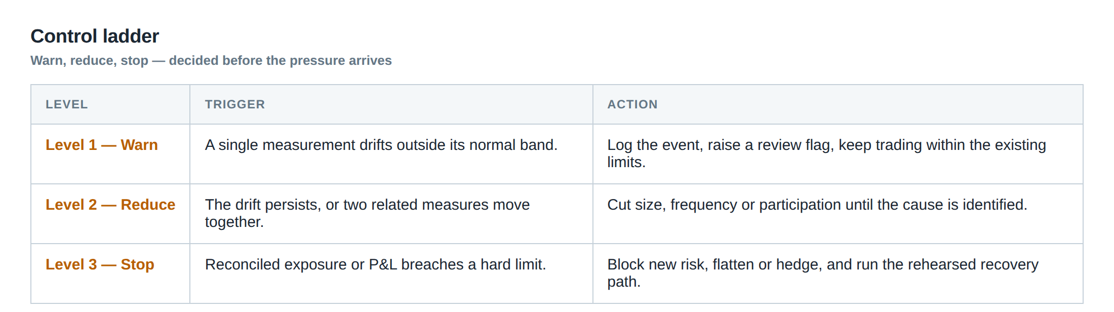
Preventative controls sit upstream of the execution engine. A pre‑trade inventory buffer ensures that a minimum number of contracts are always resident on the “sell” venue, reducing reliance on real‑time withdrawals. Dynamic fee‑adjustment tables flag any venue whose taker fee exceeds a configurable proportion of the observed spread, automatically disabling the arbitrage pair. Latency‑budget monitors track the round‑trip time of the settlement pipeline; if the observed latency drifts beyond a threshold, the system throttles the order size or suspends the strategy entirely. Finally, a venue‑outage watchdog subscribes to heartbeat messages; loss of a heartbeat for more than two seconds triggers an immediate pause of all cross‑venue activity, protecting the portfolio from half‑filled legs.

How to measure whether it is working

Effectiveness is measured by the realised net‑spread after all adjustments, expressed in basis points of notional. The primary metric is the “transfer‑adjusted profit per trade”, calculated as (sell‑price – buy‑price) – (fees + rebates + funding + withdrawal‑cost). A secondary metric tracks the “execution‑depth utilisation ratio”, i.e. the proportion of the displayed depth that was actually filled. The third indicator is “transfer latency variance”, the standard deviation of the time between trade execution on the buy side and the receipt of cash on the sell side. Consistently low variance indicates that the pre‑positioned inventory and withdrawal limits are correctly calibrated. Any systematic drift in these numbers should trigger a review of the cost‑model parameters or the inventory buffer size.

The portfolio view

From a portfolio perspective, cross‑venue arbitrage is a micro‑scale hedge that reduces net exposure to systematic price risk while generating a small, repeatable alpha. However, the inventory that shuttles between venues becomes a source of intra‑day liquidity risk. If the strategy accumulates a net long position on Exchange A because the sell leg repeatedly fails, the portfolio’s beta tilts upward, exposing it to market moves that the arbitrage logic does not capture. Conversely, a persistent net short on Exchange B can increase funding costs and trigger margin calls. Portfolio managers therefore monitor the net position per venue as a separate risk factor, applying VaR limits to each venue’s inventory and rebalancing with unrelated directional trades when the net exposure breaches the pre‑set thresholds. The goal is to keep the arbitrage activity self‑contained: the profit from each pair should offset the cost of holding the temporary imbalance, ensuring that the overall portfolio remains market‑neutral.

In practice, the decision to enter a cross‑venue arbitrage is a conditional probability problem: the probability that the price gap survives the full chain of transfer steps multiplied by the expected net‑spread, compared against the opportunity cost of capital tied up in pre‑positioned inventory. When the combined probability‑adjusted expected profit falls below the internal hurdle rate, the trade is rejected, even if the raw quote gap looks attractive.

The research that underpins this approach treats electronic markets as price‑time‑priority queues. It separates the value of a queue position into two components: the expected capture of the spread and the adverse‑selection cost of being front‑run. A third, often overlooked, component is the option value of retaining a place in line – the right, but not the obligation, to execute later if the spread widens further. The practical implication is that an order’s lifetime cannot be judged solely by elapsed clock time; the system must continuously reassess whether the remaining queue position, the expected spread, and the adverse‑selection risk still justify keeping the order alive. This dynamic reassessment is precisely what the transfer‑feasibility engine performs in a live arbitrage system.

Do you currently monitor the full transfer pipeline – from executable depth through settlement latency – before flagging a price gap as an arbitrage opportunity?

About the research behind this lesson

The seminar frames electronic markets as price-time-priority queues. It separates queue value into spread capture versus adverse-selection cost and the option value of retaining a place in line.

Applied to this lesson: An order lifetime therefore cannot be based on elapsed time alone: the system must reassess whether its queue position, expected spread and adverse-selection risk still justify keeping the order alive.

Two live systems, one desk

PULSE-X — power-packed HFT: high-frequency momentum on XAUUSD and EURUSD. System details · Live account

NIC-X — ultra-low drawdown: displaced-print arbitrage for large capital. System details · Live account

Start now: leave your email and request a free trial — we will send the pricing, the connection route and the trial terms. Pricing

Join the market discussion: Telegram @squawklive

Source: High-Frequency Trading and Modern Market Microstructure

Educational content only. Trading leveraged products involves risk.