October 5, 2026

What this problem really is

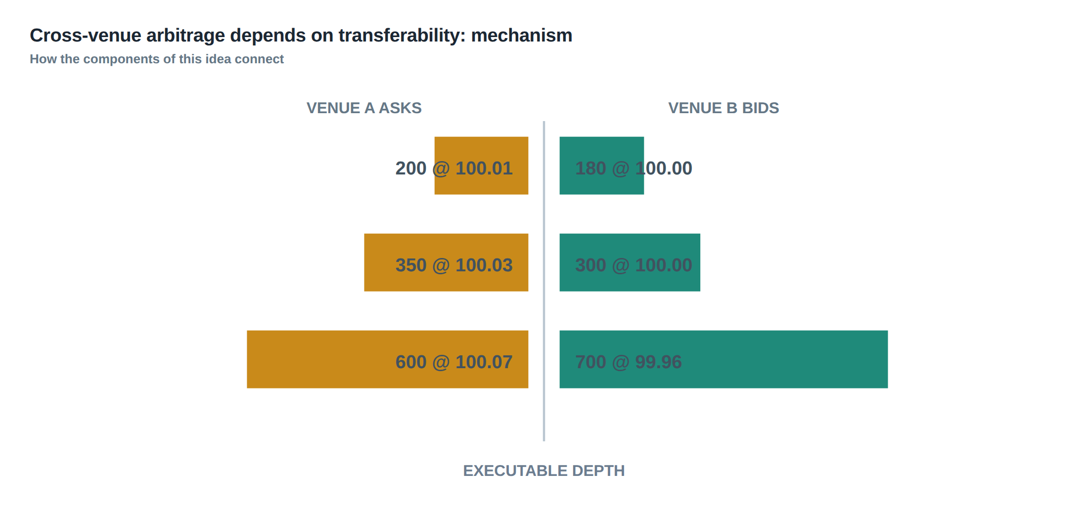
Cross‑venue arbitrage is often described as “buy at the bid on Venue A, sell at the ask on Venue B”. In practice the two displayed prices are only the tip of a deeper queue. The tip may be thin, may be protected by maker‑rebate rules, or may be inaccessible because the trader does not hold the required inventory on the right side of the market. When the underlying order‑book depth, settlement timelines, or withdrawal limits differ between venues, the apparent price gap can evaporate before any trade is executed.

The difficulty is therefore not a lack of price disparity but a mismatch between the executable depth of the two books and the operational constraints that bind the trader’s capital. If the buy leg can be filled only at a price deeper than the displayed bid, or if the sell leg is subject to a withdrawal freeze, the theoretical spread is never realised. The arbitrageist must treat the two legs as a single contingent transaction whose feasibility depends on inventory location, funding cost, and venue‑specific rules.

A naïve strategy that posts a market order on the cheap side and a limit order on the expensive side will frequently fail when the market moves, when fees and rebates are applied, or when the settlement window of the cheap venue lags the expensive one. The core thesis is that “two displayed prices are not one executable arbitrage unless inventory, settlement and venue rules allow both legs to complete”. The remainder of this article unpacks that thesis in operational detail.

How the mechanism works, step by step

The first step is to map the executable depth of each venue. This means extracting not only the best‑bid and best‑ask but also the cumulative volume available at each price level down to a depth where the marginal profit after fees becomes zero. The depth curve is a function of the order‑book shape and of any maker‑rebate schedule that may turn a nominal spread into a net loss for a taker.

Second, the trader must overlay the funding and withdrawal constraints that apply to the cash or securities required for each leg. Some venues settle on a T+0 basis, others on T+2, and a few impose a minimum balance that cannot be withdrawn within a defined window after a trade. These constraints translate into an opportunity cost that can be expressed as a financing rate applied to the notional that remains tied up on the “cheap” side while the “expensive” side is being cleared.

Third, the system must evaluate inventory placement. If the cheap side requires the trader to own the asset before the trade can be executed, but the asset is currently held on the expensive side, a pre‑positioning transfer is needed. The transfer latency—whether it is an internal ledger move or a cross‑border settlement—must be compared with the expected lifetime of the arbitrage window. If the transfer takes longer than the window, the arbitrage is effectively unavailable, and the order should be cancelled before it reaches the market.

Only after these three layers—executable depth, funding/withdrawal constraints, and inventory location—have been reconciled can the algorithm compute a net spread that survives all costs and timing risks. The decision to send a pair of orders is then based on a deterministic inequality rather than a simple price‑difference threshold.

A worked example with real numbers

Consider a futures contract that trades on two electronic venues, Alpha and Beta. Alpha shows a best bid of 9 950 USD with 200 contracts available, and a second‑level bid of 9 940 USD with 1 500 contracts. Beta displays a best ask of 9 970 USD with 300 contracts, and a second‑level ask of 9 980 USD with 2 000 contracts. The maker‑rebate on Alpha is –0.2 USD per contract for taker orders, while Beta offers a +0.1 USD rebate for maker orders. Transaction fees are 0.05 USD on Alpha and 0.03 USD on Beta.

A naïve spread calculation would take the top‑of‑book numbers: 9 970 – 9 950 = 20 USD per contract, apparently a tidy arbitrage. After applying fees, the net becomes 20 – 0.05 – 0.03 = 19.92 USD. However, the taker on Alpha must pay the –0.2 USD rebate, reducing the profit to 19.72 USD. Moreover, the trader only holds 100 contracts on Alpha, insufficient to fill the 300‑contract ask on Beta. The executable depth on Alpha at the 9 950 level is 200 contracts, but the net profit per contract at that level, after fees and rebate, is 19.72 USD. To capture the full 300‑contract ask on Beta, the trader would need to buy 300 contracts on Alpha, which forces the order down to the 9 940 level where the spread collapses to 30 USD (9 970 – 9 940) before fees, yielding a net of 30 – 0.05 – 0.03 – 0.2 = 29.72 USD per contract. The total profit would be 300 × 29.72 = 8 916 USD, but the required cash on Alpha is 300 × 9 940 = 2 982 000 USD, which exceeds the trader’s allocated capital on that venue by 2 882 000 USD.

Compounding the issue, Beta settles on a T+2 schedule, while Alpha settles instantly. The trader’s cash would therefore be tied up on Alpha for two days, incurring a financing cost of 0.015 % per day on the notional, amounting to roughly 447 USD over the holding period. Subtracting this from the gross profit leaves 8 469 USD, still positive but now sensitive to any slippage on the second‑level bid. If the market moves 5 USD against the trader before the order is filled, the net profit evaporates. The example demonstrates that a quoted price gap can disappear after fees, financing, and inventory constraints are applied, and that the arbitrage is only viable when the trader can pre‑position the required contracts on the cheap venue faster than the window closes.

Where it breaks in live markets

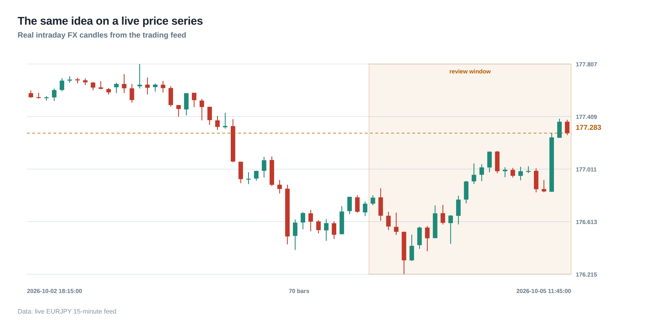
In a live environment the most common failure mode is the queue‑decay effect. The moment a large taker order is placed on the cheap side, other participants may react, moving the price deeper into the book or cancelling their own orders to protect against adverse selection. The research on price‑time‑priority queues shows that the value of a queue position consists of the captured spread, the cost of being picked off by better‑informed traders, and the optionality of staying in line. When the expected adverse‑selection cost rises faster than the spread, the queue position becomes a liability, and the order is often withdrawn automatically.

A second failure point is venue‑specific withdrawal limits. Some platforms impose a “cool‑down” period after a trade during which the newly acquired inventory cannot be moved out of the venue. If the arbitrage window is shorter than this period, the second leg cannot be executed, and the trader is left with an unhedged position that may incur market risk.

Third, funding mismatches can render an otherwise profitable spread negative. High‑frequency traders often obtain ultra‑low‑cost financing through internal repo lines, but a prop desk may be constrained by external funding rates that fluctuate throughout the day. When the financing cost of holding the cheap‑side inventory exceeds the gross spread, the arbitrage becomes a loss.

Finally, systemic outages such as a temporary loss of connectivity to one venue can freeze the ability to cancel or modify orders. If a buy order on Alpha is filled while the sell order on Beta cannot be sent because of an outage, the trader ends up with a naked long exposure. The risk of such “partial fill” events must be built into the control framework.

The operating path, stage by stage

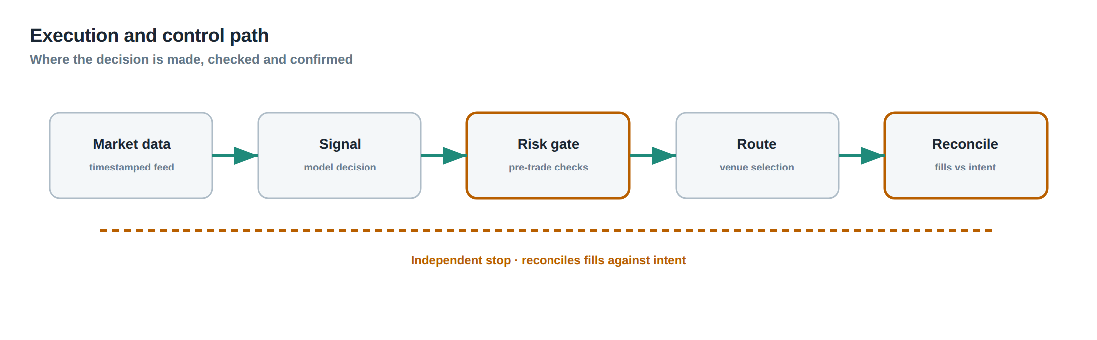
Stage 1 is market data ingestion. The system subscribes to depth‑of‑book feeds from all relevant venues, normalises timestamps, and builds a real‑time executable‑depth map that includes cumulative volume at each price level.

Stage 2 is constraint overlay. For each venue the engine retrieves the current funding rate, settlement lag, and any withdrawal freeze flags. It also queries the internal ledger for the location of inventory, distinguishing between settled cash, unsettled cash, and tokenised positions.

Stage 3 is spread computation. The algorithm subtracts explicit fees, rebates, and the estimated financing cost for the projected holding period from the raw price difference. It then checks whether the cumulative volume at the adjusted price level on the cheap side meets or exceeds the volume needed on the expensive side.

Stage 4 is pre‑positioning decision. If the required inventory is not present on the cheap venue, the engine calculates the transfer latency—whether an internal ledger move (sub‑millisecond) or an external settlement (seconds to minutes). If the latency exceeds the projected arbitrage window, the opportunity is discarded.

Stage 5 is order placement and monitoring. The system sends a pair of orders, typically a taker order on the cheap side and a maker order on the expensive side, with explicit time‑in‑force parameters that match the expected window. Continuous monitoring of queue position, market movement, and venue health feeds back into a dynamic risk‑adjusted stop‑loss that can cancel both legs if the net spread deteriorates.

Stage 6 is post‑trade reconciliation. Once both legs have cleared, the engine settles the cash flows, updates the internal inventory map, and records the realised profit after all costs. If only one leg filled, a contingency routine initiates a hedge or a forced unwind to limit exposure.

Each stage must be executed within a deterministic latency budget; otherwise the arbitrage window may close before the order reaches the market. The flow diagram in the next figure summarises this pipeline.

Controls that act before the damage

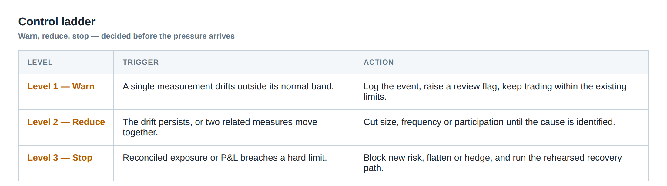
The first line of defence is a pre‑trade eligibility filter that checks inventory location, funding rate, and venue‑specific withdrawal flags before any order is generated. If the filter flags a mismatch, the algorithm aborts the trade and logs the reason for later analysis.

A second control is the dynamic queue‑value monitor. By continuously re‑evaluating the expected spread, adverse‑selection cost, and the optionality of staying in line, the system can withdraw an order the moment the net expected value falls below a pre‑set threshold. This is a direct operational translation of the research insight that order lifetime cannot be judged solely by elapsed time; the queue’s economic value must be re‑assessed at each tick.

A third safeguard is the transfer‑latency guard. The engine maintains a rolling estimate of internal and external transfer times based on recent observations. If the estimated time to move the required contracts exceeds the projected arbitrage window, the guard prevents order submission and optionally triggers a pre‑emptive inventory rebalance to bring the needed volume onto the cheap venue.

Finally, a venue‑outage detector watches heartbeat messages and order‑acknowledgement latencies. When a venue’s feed stalls or acknowledgements are delayed beyond a configurable threshold, the detector suspends any pending orders that involve that venue and initiates a rapid unwind of any partially filled legs. The ladder diagram in the following figure illustrates how these controls stack to protect the portfolio.

How to measure whether it is working

Effectiveness is measured by the net realised spread per executed arbitrage, expressed in basis points of notional after all fees, rebates, and financing costs. A useful benchmark is the expected spread computed at the moment of order entry; the ratio of realised to expected spread indicates how often the queue‑value model accurately predicts execution.

Another metric is the fill‑rate differential between the cheap‑side taker order and the expensive‑side maker order. A high differential suggests that inventory or transfer constraints are causing partial fills, which should be reflected in a higher incidence of forced hedges.

The average latency of pre‑positioning transfers is also tracked. If the observed transfer time consistently exceeds the arbitrage window, the system should be re‑engineered to either widen the window or increase pre‑positioned inventory.

Finally, the incidence of venue‑outage‑related partial fills is logged. A rising trend signals the need for redundancy in data feeds or for tighter heartbeat thresholds. By aggregating these statistics over a rolling window of, say, 10 000 arbitrage attempts, the desk can quantify the proportion of opportunities that were lost purely to operational frictions rather than market inefficiency.

The portfolio view

From a portfolio perspective, cross‑venue arbitrage is a zero‑beta strategy that should add a small, steady stream of return while leaving the overall market exposure unchanged. However, the operational constraints discussed above introduce latent risk that manifests as occasional directional exposure when only one leg of the trade executes.

The risk manager must therefore treat the arbitrage desk as a micro‑portfolio with its own capital allocation, funding cost curve, and liquidity buffer. The allocated capital should be sufficient to cover the worst‑case scenario of a full‑size buy on the cheap side that cannot be hedged because of a venue outage. Stress‑testing should include scenarios where transfer latency spikes to several minutes, where fees are doubled due to a temporary promotion change, and where a sudden withdrawal freeze locks inventory for an entire trading session.

By aggregating the net realised spread across all venues and normalising by the capital at risk, the desk can compute an operational Sharpe ratio that isolates the pure execution skill from market‑driven alpha. Monitoring this ratio over time reveals whether the control framework is maintaining the intended risk‑return profile or whether hidden frictions are eroding profitability.

In practice, the desk will also overlay the arbitrage returns on top of its broader market‑neutral or directional positions, ensuring that any residual exposure from a failed arbitrage does not compound with existing risk factors. The final step is to feed the performance data back into the pre‑trade filter, tightening thresholds where the realised spread consistently underperforms the model, and thereby closing the loop between measurement and control.

Do you have a systematic way of quantifying the hidden cost of inventory transfer latency in your own cross‑venue arbitrage workflow?

About the research behind this lesson

The seminar frames electronic markets as price-time-priority queues. It separates queue value into spread capture versus adverse-selection cost and the option value of retaining a place in line.

Applied to this lesson: An order lifetime therefore cannot be based on elapsed time alone: the system must reassess whether its queue position, expected spread and adverse-selection risk still justify keeping the order alive.

Explore PULSE: System details

PULSE live account: Verify the live account on FX Blue

Live chat and updates: Telegram @xtrskhft

Source: High-Frequency Trading and Modern Market Microstructure

Educational content only. Trading leveraged products involves risk.