October 12, 2026

What this problem really is

Arbitrage opportunities are rarely a single static price gap; they are a dynamic pair of execution legs that must be completed in a narrow time window. In electronic markets each leg is a standing order that lives in a price‑time‑priority queue. The “spread” that appears on a screen is the theoretical profit after both legs have been filled, but the moment the first leg is executed the trader is exposed to the risk that the second leg will not materialise, will be only partially filled, or will be filled at a worse price. The interval between the two fills therefore contains directional exposure (the market may move against the remaining leg) and liquidity exposure (the counter‑venue may run out of depth or reject the order). The problem is not simply “how fast can we hit both prices”, but “how can we continuously monitor the filled‑versus‑remaining quantities, decide when to abandon or reroute the outstanding leg, and price the cost of neutralising an unmatched position”.

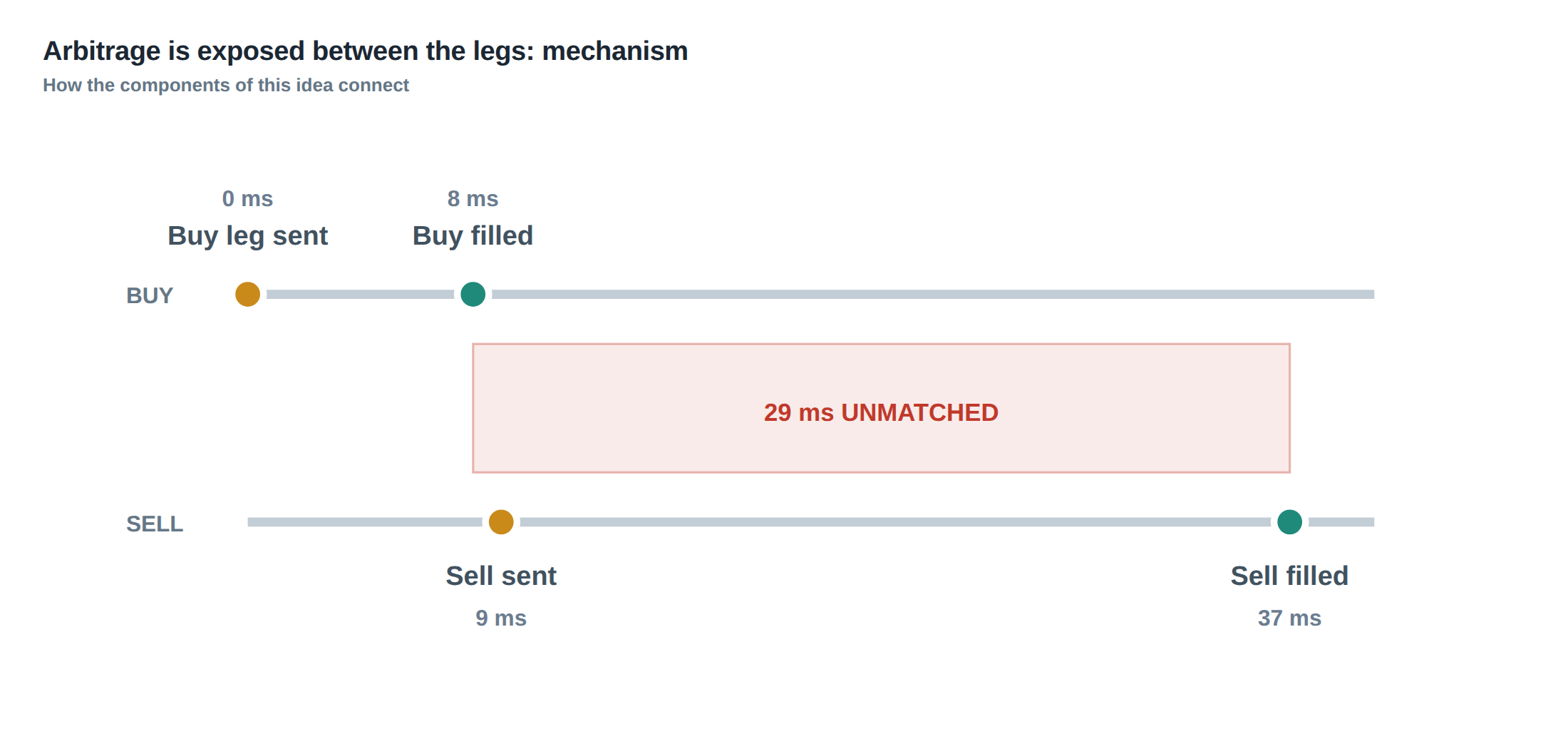
How the mechanism works, step by step

When a trader spots a cross‑venue spread, the system creates two child orders: a buy on the cheap venue and a sell on the expensive venue. Each child order carries a target quantity, a minimum execution size dictated by the venue (for example 100 shares on a dark pool) and a set of thresholds that govern its lifecycle. The first threshold is the hedge trigger – if the market moves a pre‑specified fraction of the spread (say 20 bps) while the order is still open, the system flags the leg as “at risk”. The second is the cancel trigger, a larger adverse move (for instance 50 bps) beyond which the order is withdrawn outright. A third, more subtle, reroute trigger activates when the expected fill probability falls below a calibrated level (for example 30 % based on recent venue latency and depth).

At every market event – a new quote, a trade, a depth change – the engine recomputes the filled quantity and the remaining quantity for each leg. If a partial fill occurs, the remaining quantity is reduced, but the exposure does not vanish; the unfilled portion still carries the same directional risk, now amplified because the realised profit on the filled portion is locked in while the unfilled side is still open. The system therefore updates a “completion‑time distribution” for the outstanding leg, using historic latency and fill‑rate data to estimate the probability of finishing within a given horizon. If the probability of completing before the next expected price move drops below a pre‑set confidence level (often 70 % for high‑frequency desks), the reroute logic may divert the remaining quantity to an alternative venue with a deeper queue or a different order type.

The final step is the neutralisation decision. Should the outstanding leg be cancelled, the trader must unwind the already‑filled leg, which turns the theoretical spread into a realised directional position. The cost of this unwind is measured in basis points of the original spread and includes the market impact of crossing the spread in the opposite direction, the opportunity cost of the missed arbitrage, and any fees associated with the cancellation.

A worked example with real numbers

Consider a prop‑trading desk that monitors the EUR/USD futures market on two ECNs. On ECN‑A the best ask is 1 250.00 USD, while on ECN‑B the best bid is 1 250.05 USD, giving a raw spread of five ticks (0.05 %). The desk decides to trade 10 000 contracts, each contract representing 100 000 EUR, so the notional is 1 billion EUR. The minimum order size on ECN‑A is 100 contracts, and the desk’s internal policy is to split the total into ten child orders of 1 000 contracts each, to avoid signalling.

The buy order on ECN‑A is submitted at 1 250.00 USD with a hedge threshold of 2 bps (0.02 %) and a cancel threshold of 5 bps. The sell order on ECN‑B is placed at 1 250.05 USD with identical thresholds. Within 120 ms the buy order receives a partial fill of 600 contracts; the remaining 400 contracts sit in the queue. The sell order, however, suffers a sudden withdrawal of depth on ECN‑B: the best bid drops to 1 250.02 USD and the displayed depth at 1 250.05 USD evaporates. The order engine records a zero fill after 150 ms and updates the completion‑time distribution for the sell leg: the historic 95th‑percentile fill time for a 1 000‑contract order on ECN‑B is 350 ms, but the current market depth suggests a probability of only 22 % of completing within that horizon.

Because the probability falls below the reroute trigger (30 %), the system automatically cancels the original sell order and resubmits a marketable order for the remaining 1 000 contracts on ECN‑C, where the best bid is now 1 250.01 USD and the minimum order size is 50 contracts. The marketable order executes immediately at 1 250.01 USD, incurring a cost of 4 ticks relative to the original target.

At this point the desk holds a long position of 600 contracts bought at 1 250.00 USD and a short position of 1 000 contracts sold at 1 250.01 USD, leaving a net exposure of +400 contracts (long). The market continues to move against the long side; within the next 200 ms the price drops to 1 249.80 USD, a 20‑tick adverse move. To neutralise the exposure the desk must sell the 400 contracts at the prevailing bid of 1 249.80 USD, realising a loss of 20 ticks on the unmatched leg. Relative to the original five‑tick spread, the net result is a loss of 15 ticks, equivalent to 0.12 % of notional, or roughly 120 bps when expressed as a basis‑point cost of the attempted arbitrage.

The example illustrates how the interval between the first fill and the completion of the second leg can transform an apparently risk‑free spread into a directional position that is liquidated at the worst possible market moment.

Where it breaks in live markets

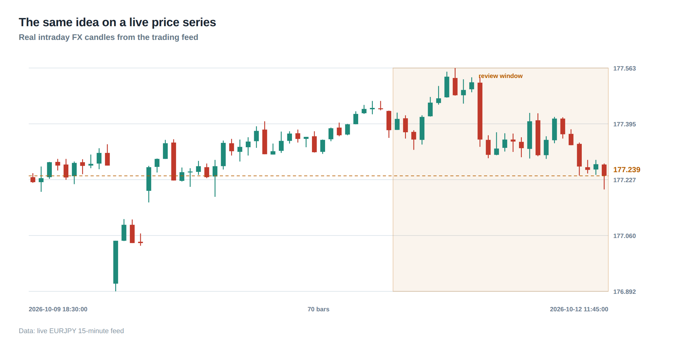
In theory the thresholds and reroute logic described above should protect the desk from most adverse outcomes, but live markets introduce several failure modes. First, latency spikes are not uniformly distributed; a sudden surge in network traffic can add 200 ms or more to the round‑trip time, pushing a high‑probability fill into the tail of the completion‑time distribution. Second, venue‑specific minimum order sizes can create “granularity gaps”. If a venue enforces a 500‑contract minimum, a desk that has already filled 300 contracts cannot submit a residual order without either over‑exposing itself or waiting for additional market depth to accumulate. Third, hidden liquidity and iceberg orders mean that the displayed depth may be a poor proxy for true fill probability, especially when large institutional participants withdraw hidden orders in response to a perceived arbitrage. Fourth, the assumption of independent legs breaks down when the two venues share the same liquidity pool; a large execution on one side can immediately deplete the opposite side, causing the second leg to disappear in the same millisecond that the first leg is filled.

Finally, the cost of neutralising an unmatched leg is often underestimated because market impact is non‑linear. Selling a large residual position into a thin order book can move the price several ticks further than the simple spread differential suggests, especially in volatile periods where the order book thins dramatically. The combination of these factors means that even a well‑tuned algorithm can be caught out by a confluence of latency, granularity, hidden liquidity, and impact.

The operating path, stage by stage

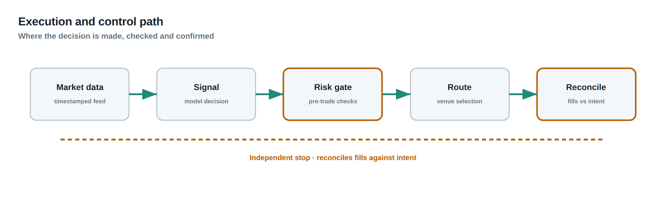
The desk’s execution engine follows a deterministic flow that can be visualised as a ladder of decision points. The first rung is opportunity detection, where a cross‑venue price differential exceeding the pre‑trade profitability threshold is flagged. The second rung is order construction, during which the target quantity is split, venue‑specific minimums are applied, and the hedge, cancel, and reroute thresholds are attached to each child order. The third rung is real‑time monitoring, where every market event triggers an update of filled versus remaining quantity, a recomputation of the completion‑time distribution, and a check against the three thresholds. The fourth rung is adaptive response, where the engine may reroute, amend, or cancel the outstanding leg based on the latest risk metrics. The fifth rung is post‑trade reconciliation, where the realised P&L is compared with the theoretical spread and the cost of any neutralisation is recorded. The final rung is feedback integration, feeding the observed fill times, partial‑fill frequencies, and impact costs back into the statistical models that drive the thresholds.

Each stage must be executed within a deterministic sub‑millisecond budget to avoid cascading delays. The monitoring stage, for example, must process depth updates from multiple venues in parallel, apply a Kalman‑filter‑like estimator to the completion‑time distribution, and output a binary decision (continue, reroute, cancel) before the next market tick arrives. Any breach of this budget creates a hidden latency that effectively widens the interval between legs, increasing exposure.

Controls that act before the damage

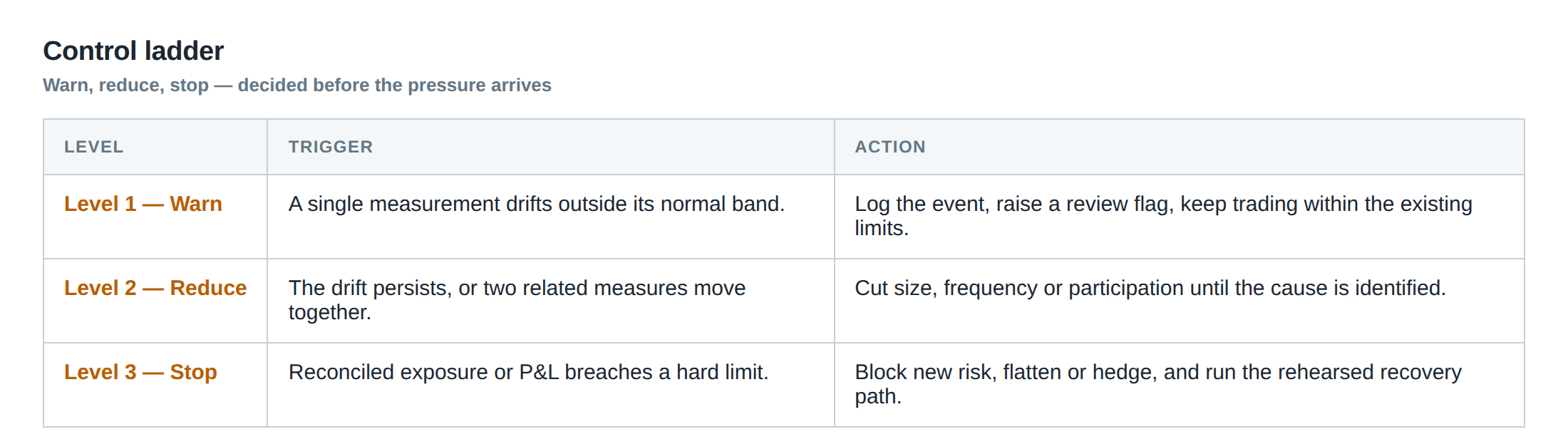
Preventive controls are layered to catch the problem before the unmatched leg becomes a material loss. The first layer is pre‑trade validation, which checks that the combined minimum order sizes of both legs do not exceed the intended trade size; if they do, the trade is rejected or the size is reduced to the nearest feasible multiple. The second layer is real‑time exposure caps, which limit the net open quantity of any single arbitrage strategy to a fraction of the desk’s capital, ensuring that a single failure cannot blow out the balance sheet. The third layer is dynamic threshold calibration, where the hedge, cancel, and reroute thresholds are continuously adjusted based on rolling windows of latency and fill‑rate statistics; a sudden increase in average latency automatically tightens the cancel threshold. The fourth layer is venue health monitoring, which tracks heartbeat messages, order‑rejection rates, and depth‑refresh latency for each venue; a degradation beyond a pre‑set tolerance triggers an automatic suspension of new orders to that venue. The final layer is stress‑test simulation, run every shift, that injects synthetic latency spikes and depth withdrawals into the live order flow to verify that the reroute and cancel logic behaves as expected under extreme conditions.

These controls are not static check‑boxes; they are part of an adaptive feedback loop that learns from each execution. When a neutralisation event occurs, the system records the price at which the residual leg was liquidated, the time elapsed since the first fill, and the reason for the failure (e.g., depth disappearance, latency spike). This data feeds the next calibration cycle, tightening thresholds where necessary and relaxing them where the market proves robust.

How to measure whether it is working

Performance measurement must separate the pure spread capture from the cost of the protective mechanisms. The primary metric is net spread realised, calculated as the sum of the executed buy price and sell price across both legs, minus the theoretical spread that existed at the moment of detection. This figure is then adjusted for neutralisation loss, the P&L impact of any residual position that had to be closed at an adverse price. A second metric is completion‑time success rate, the proportion of legs that finish within the predicted 95th‑percentile window; this should be tracked per venue and per order size.

A third, more diagnostic, measure is threshold breach frequency: how often the hedge or cancel thresholds are triggered, and whether the subsequent actions (reroute, cancel) prevented a larger loss. The fourth metric is impact‑adjusted cost, derived from a market‑impact model that estimates the price move caused by the neutralising trade relative to the prevailing order book depth. Finally, system latency budget adherence is monitored by timestamping each event from market data receipt to order‑state update; any deviation beyond the allocated sub‑millisecond budget is flagged for investigation.

Together these metrics give a multi‑dimensional view of the system’s health: a high net spread with low neutralisation loss indicates that the protective thresholds are well‑tuned, whereas a high breach frequency combined with frequent neutralisation losses points to either overly aggressive spread hunting or a deteriorating venue environment.

The portfolio view

From a portfolio perspective the arbitrage leg is a micro‑position that sits alongside the desk’s broader directional exposures. Because the unmatched leg can temporarily become a directional bet, the desk must incorporate its potential impact into the overall risk‑budget. This is achieved by treating the residual quantity as a temporary delta that is added to the net market exposure for the duration of the execution window. The delta is weighted by the probability of completion, producing an expected exposure that can be hedged with a small futures position or an options overlay if the desk’s risk appetite permits.

When the execution completes, the temporary delta is removed and the realised P&L is booked. Over a rolling horizon the desk tracks the arbitrage turnover ratio, the proportion of total notional that passes through cross‑venue spreads, and the risk‑adjusted return, which divides the net spread realised by the maximum temporary delta ever held. A healthy arbitrage engine will show a high turnover ratio with a modest temporary delta, indicating that the desk is efficiently converting fleeting price gaps into profit without materially altering its market‑directional stance.

In practice, the portfolio manager will set a ceiling on the aggregate temporary delta across all arbitrage strategies, ensuring that the desk’s net market exposure never exceeds the limits set for the core directional book. The manager also monitors the correlation between arbitrage execution times and macro‑level market moves; if the desk consistently finds itself long when the market is falling, the correlation may suggest a systemic latency bias that needs to be corrected.

—

Do you have a systematic way to monitor the live probability that each leg of a spread will finish before the market moves against you?

About the research behind this lesson

The seminar frames electronic markets as price-time-priority queues. It separates queue value into spread capture versus adverse-selection cost and the option value of retaining a place in line.

Applied to this lesson: An order lifetime therefore cannot be based on elapsed time alone: the system must reassess whether its queue position, expected spread and adverse-selection risk still justify keeping the order alive.

Explore PULSE: System details

PULSE live account: Verify the live account on FX Blue

Live chat and updates: Telegram @xtrskhft

Source: High-Frequency Trading and Modern Market Microstructure

Educational content only. Trading leveraged products involves risk.