October 13, 2026

What this problem really is

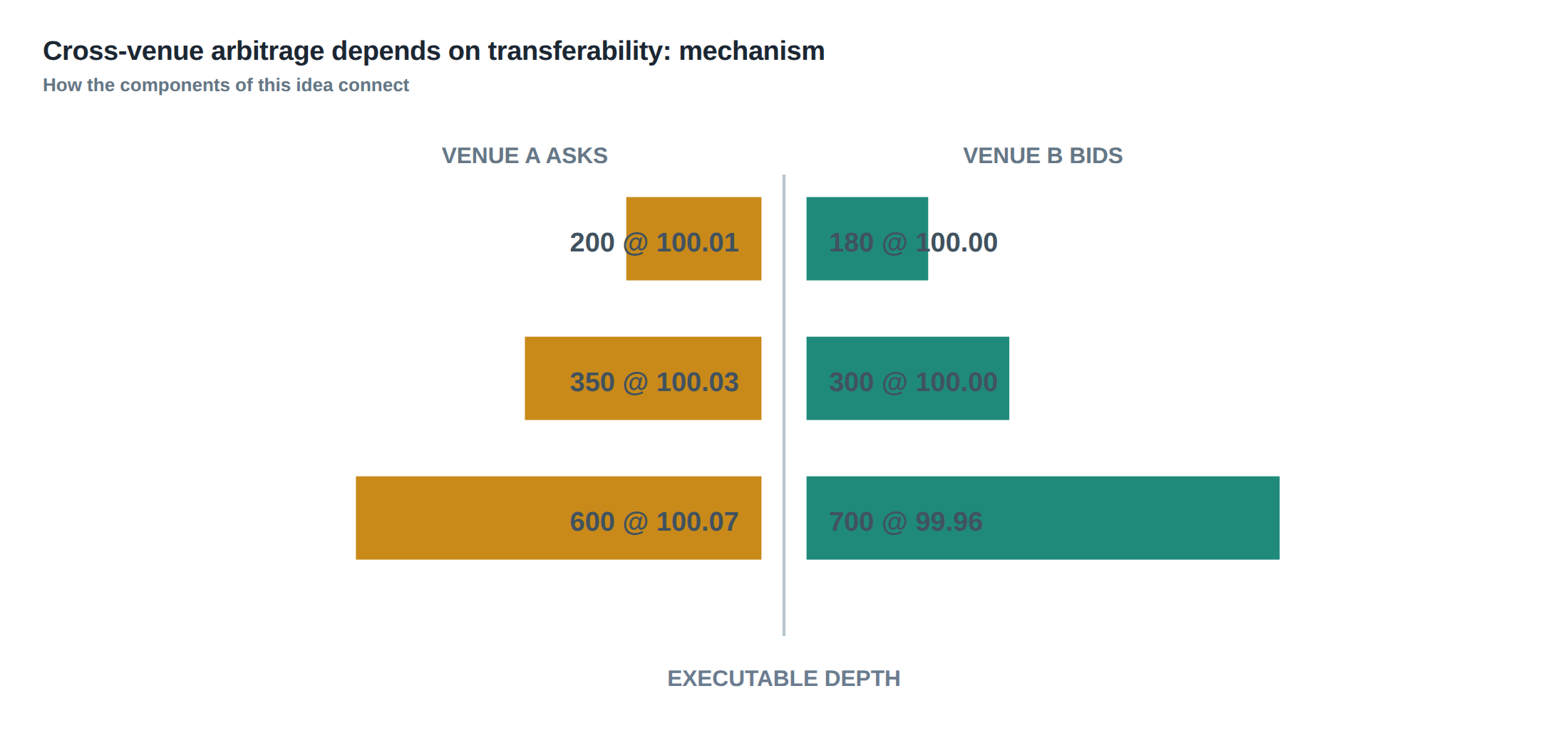
The term cross‑venue arbitrage is often reduced to “buy low on Exchange A, sell high on Exchange B”. In practice the two quoted prices are only the tip of a much deeper order‑book structure. The visible best bid and ask may sit on a thin slice of liquidity that cannot be filled without moving the price, and the apparent spread can disappear once the full cost of execution is accounted for. Moreover, the two legs of the trade are subject to distinct settlement cycles, margin requirements, and withdrawal constraints. If the trader does not possess the necessary inventory on the selling venue, or cannot transfer cash fast enough to fund the purchase, the displayed price gap never becomes a real, executable arbitrage. In short, the arbitrage exists only when the combined operational and financial frictions are low enough for both legs to close simultaneously.

The problem is therefore not a question of “price mismatch” alone but a multi‑dimensional feasibility test: depth at each venue, fee and rebate schedules, funding latency, and the rules governing the movement of securities and cash across venues. When any of these dimensions is restrictive, the theoretical profit evaporates before the order can be filled. The trader must therefore treat the arbitrage opportunity as a conditional contract that expires the instant any prerequisite fails.

How the mechanism works, step by step

The first step is to retrieve the full depth of the order book on each venue, not merely the top‑of‑book quotes. A realistic model will sum the available volume at each price level until the desired trade size is reached, thereby producing an executable depth curve. The second step is to overlay the explicit transaction costs – exchange fees, maker‑taker rebates, and any clearing or settlement charges – on each leg of the trade. Third, the trader must map the cash‑to‑security conversion path, accounting for the time required to move funds from the account that will fund the buy to the account that will receive the proceeds of the sell.

If the transfer time exceeds the window in which the price gap persists, the trader must decide whether to pre‑position inventory on the selling venue. Pre‑positioning carries its own cost: capital is tied up, and the trader is exposed to adverse price movement while waiting for the arbitrage trigger. The final step is a risk‑adjusted profitability check that includes the probability of venue outage, the counter‑party exposure during the settlement window, and the optionality value of retaining a place in the queue. If the net expected profit after all adjustments is positive, the order is released; otherwise it is cancelled.

A worked example with real numbers

Consider a futures contract that trades on Venue X and Venue Y. Venue X shows a bid of 10 200 USD with 5 contracts available at that price, then 10 190 USD for the next 10 contracts. Venue Y displays an ask of 10 150 USD with 8 contracts at that level, followed by 10 140 USD for the next 12 contracts. The trader wishes to execute a 12‑contract arbitrage.

On Venue X the executable sell price is calculated by filling the top 5 contracts at 10 200 and the remaining 7 contracts at 10 190, giving an average sell price of (5 × 10 200 + 7 × 10 190) / 12 = 10 196 USD. On Venue Y the executable buy price uses the first 8 contracts at 10 150 and the next 4 at 10 140, yielding an average buy price of (8 × 10 150 + 4 × 10 140) / 12 = 10 147 USD. The raw spread before fees is therefore 49 USD per contract.

Venue X charges a taker fee of 0.02 % and offers a maker rebate of 0.03 % for limit orders that add liquidity. Since the sell order will hit the existing bid, the taker fee applies: 10 196 × 0.0002 ≈ 2.04 USD per contract. Venue Y applies a maker rebate of 0.03 % because the buy order will sit at the best ask: 10 147 × 0.0003 ≈ 3.04 USD per contract. Adding clearing fees of 0.5 USD per leg, the total cost per round‑trip contract becomes 2.04 + 3.04 + 1.0 = 6.08 USD. The net profit before financing is therefore 49 – 6.08 ≈ 42.92 USD per contract, or about 515 USD for the 12 contracts.

However, the trader’s cash sits in a margin account linked to Venue X, while the buying power on Venue Y is limited by a 2‑hour withdrawal lock. The transfer of 12 × 10 147 ≈ 121 764 USD would therefore not be available in time to fund the purchase. The trader can either pre‑position the cash on Venue Y, incurring an opportunity cost equal to the financing rate (say 3 % annualised, or roughly 0.25 % for a 2‑hour window, i.e. ≈ 30 USD), or accept that the arbitrage will fail if the price gap closes before the funds arrive.

Assuming the trader pre‑positions the cash, the adjusted profit becomes 515 – 30 ≈ 485 USD, still attractive. If instead the trader attempts to fund the buy after the sell, the 2‑hour latency means the price gap would likely have narrowed; historical micro‑price decay suggests a 0.3 % contraction over that interval, wiping out the spread. This example shows that the quoted gap can vanish after fees, or remain unreachable because capital is locked on the wrong venue.

Where it breaks in live markets

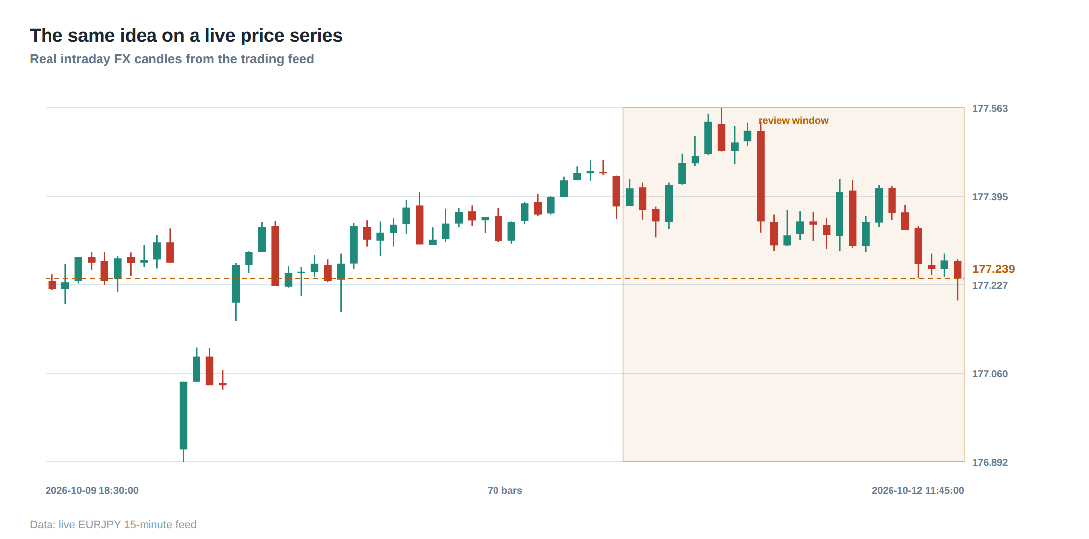
In a live environment the assumptions that underpin the worked example are constantly tested. First, depth can evaporate in milliseconds when a large hidden order is revealed, or when a market‑making algorithm pulls liquidity in response to a perceived arbitrage attempt. Second, fee schedules are not static; some venues waive taker fees for high‑frequency participants, while others introduce dynamic rebates that depend on the proportion of total volume. Third, funding and withdrawal constraints are subject to operational risk: a delay in the clearing house’s settlement cycle, a temporary freeze on withdrawals due to regulatory scrutiny, or a network outage can all prevent cash from reaching the intended venue in time.

Venue outages are particularly pernicious. If Venue Y suffers a brief disconnection, the sell order placed on Venue X may be executed, leaving the trader short on the contract with no immediate avenue to close the position. Counter‑party exposure then rises sharply, as the trader must source the contract in the secondary market at an unknown price, potentially at a loss. Moreover, the option value of staying in the queue – the right to capture a future spread – can be eroded if the queue position is lost during the outage, turning a previously valuable limit order into a market order that pays the full taker fee.

These frictions mean that a simple “price‑difference” signal is insufficient. The trader must continuously monitor depth, fee changes, and the health of the connectivity stack, and must be prepared to abort the strategy the moment any prerequisite fails.

The operating path, stage by stage

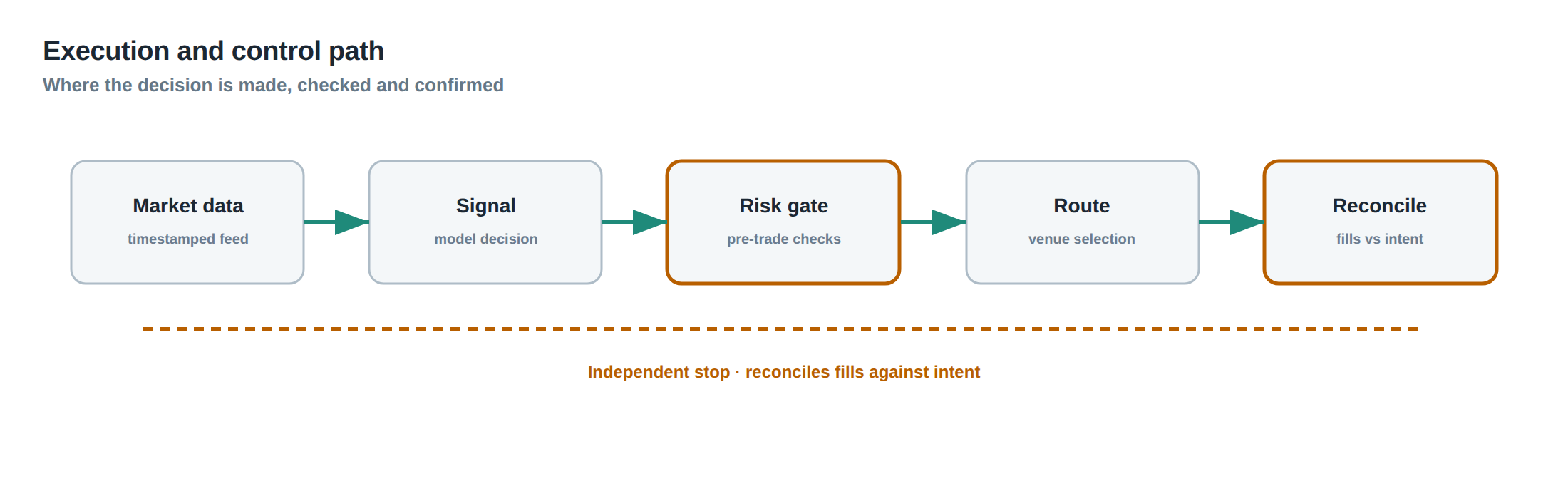
The operational workflow begins with a market‑data snapshot that includes the top 10 price levels on each venue. The system then computes the executable depth for the intended size, applying the venue‑specific fee and rebate schedule to obtain a net spread. A separate module evaluates the funding pipeline: it checks the available cash, the withdrawal lock period, and the expected settlement latency for each leg. If the funding check fails, the system either flags the opportunity for pre‑positioning or discards it.

Assuming the funding check passes, the order manager places a passive limit order on the buying venue to capture the best ask, and a marketable order on the selling venue to guarantee execution. Both orders are linked so that a fill on one side triggers a cancellation on the other if the spread collapses. A watchdog process monitors venue health; any detected outage or latency spike forces an immediate unwind of the open leg, using the best available price on the remaining venue. Finally, a post‑trade reconciler records the realised P&L, the actual fees paid, and any slippage relative to the pre‑trade executable depth calculation.

Controls that act before the damage

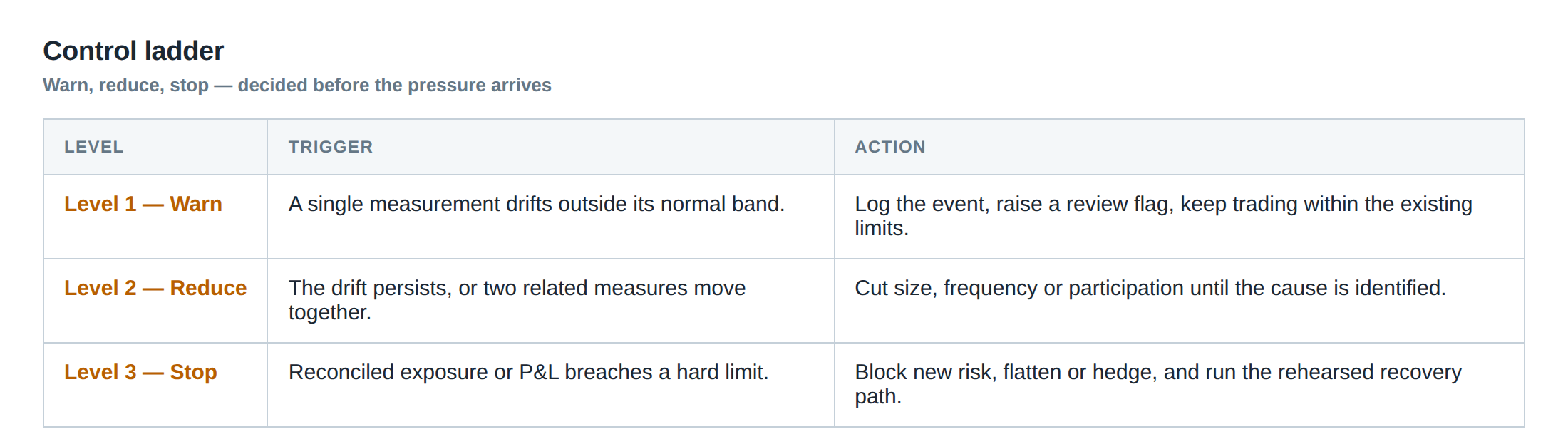
Preventive controls are layered at the data, risk, and execution tiers. At the data layer, sanity checks reject depth snapshots that show implausibly thin liquidity relative to recent averages, preventing the system from acting on stale or corrupted quotes. At the risk layer, a pre‑trade exposure limit caps the amount of inventory that can be held on any single venue, ensuring that a sudden outage does not leave the desk over‑exposed. Funding controls enforce a minimum buffer of cash on each settlement account, and automatically trigger a pre‑positioning workflow when the projected withdrawal lock exceeds the expected arbitrage window.

Execution controls include a “queue‑value” monitor that estimates the optionality of retaining a place in the limit‑order queue. If the expected adverse‑selection cost exceeds the remaining spread, the system aborts the order before it even reaches the exchange. A latency‑budget validator checks that the round‑trip network latency plus the settlement lag remain below a configurable threshold; exceeding this threshold forces the opportunity to be discarded. Together these controls act as a safety net, catching the scenario where a displayed price gap would otherwise be pursued despite an underlying operational impediment.

How to measure whether it is working

Performance measurement must separate the pure price‑difference capture from the frictions that were successfully avoided. The primary metric is net realised spread, defined as the average sell price minus the average buy price, less all explicit costs (fees, rebates, clearing charges) and implicit costs (funding interest, opportunity cost of pre‑positioned cash). A secondary metric is execution success rate, the proportion of identified opportunities that resulted in both legs filling within the predefined latency window.

Another useful indicator is queue‑value efficiency: the ratio of the realised spread to the theoretical spread that would have been obtained if the trader could have stayed in the queue indefinitely. A value close to one signals that the system is correctly timing order entry and exit relative to adverse‑selection risk. Finally, outage loss exposure quantifies the average loss incurred when a venue disconnects after one leg has filled; tracking this over time highlights whether the pre‑positioning and funding controls are adequately sized.

The portfolio view

From a portfolio perspective, cross‑venue arbitrage is a micro‑strategy that contributes to the overall risk‑adjusted return of the desk. Its correlation with broader market moves is typically low, because the profit stems from market‑structure inefficiencies rather than directional exposure. However, the strategy does introduce liquidity and funding risk that must be reflected in the capital allocation model. The capital reserved for pre‑positioned cash reduces the amount available for other strategies, and the margin required on each venue adds to the overall leverage profile.

When aggregating performance, the desk should treat arbitrage returns as net of funding cost and report them alongside the option value of queue placement – essentially the premium paid for the right to wait for a favourable spread. By integrating these components into the same risk‑adjusted framework used for other strategies, the desk can make informed decisions about scaling the arbitrage engine, adjusting fee‑rebate thresholds, or reallocating inventory to venues with more reliable transfer mechanisms.

In practice, a well‑designed arbitrage engine becomes a source of steady, low‑volatility alpha, provided that the operational constraints – depth, fees, funding latency, and venue reliability – are continuously modelled and monitored.

Would your current infrastructure allow you to quantify and act on the true executable depth of a price gap before funding or venue constraints invalidate the trade?

About the research behind this lesson

The seminar frames electronic markets as price-time-priority queues. It separates queue value into spread capture versus adverse-selection cost and the option value of retaining a place in line.

Applied to this lesson: An order lifetime therefore cannot be based on elapsed time alone: the system must reassess whether its queue position, expected spread and adverse-selection risk still justify keeping the order alive.

Explore PULSE: System details

PULSE live account: Verify the live account on FX Blue

Live chat and updates: Telegram @xtrskhft

Source: High-Frequency Trading and Modern Market Microstructure

Educational content only. Trading leveraged products involves risk.