October 15, 2026

What this problem really is

When a systematic strategy suffers a series of losing trades, the raw number that appears on the P&L screen – “‑$2.3 m” or “‑3 % of capital” – is often treated as a diagnostic in itself. In reality the figure is only a symptom of a deeper process: a breach of the statistical expectations that underlie the model, a change in market micro‑structure, or a failure of the execution engine. The danger lies in treating the drawdown as a one‑off event and then allowing the system to self‑heal by simply increasing position size until the loss is erased. This creates a feedback loop where the same weakness that generated the loss is amplified, turning a recoverable dip into a terminal ruin.

A robust drawdown control regime recognises that the loss is a signal that the assumptions of the strategy have been violated. It therefore couples the magnitude of the loss with a set of pre‑agreed actions – warnings, partial de‑risking, full shutdown – and a disciplined recovery path that must be demonstrated before any increase in exposure is permitted. The control framework must operate at both the individual strategy level and the aggregate portfolio level, because a loss in a single high‑frequency signal can be masked by gains elsewhere if the portfolio‑wide view is ignored.

The core thesis, therefore, is that a drawdown number only becomes useful when it is embedded in a decision‑making process that forces the trader or the algorithm to act, rather than react passively. The process must be codified, back‑tested, and enforced by the technology stack, otherwise human bias will inevitably erode the discipline that the control is meant to provide.

How the mechanism works, step by step

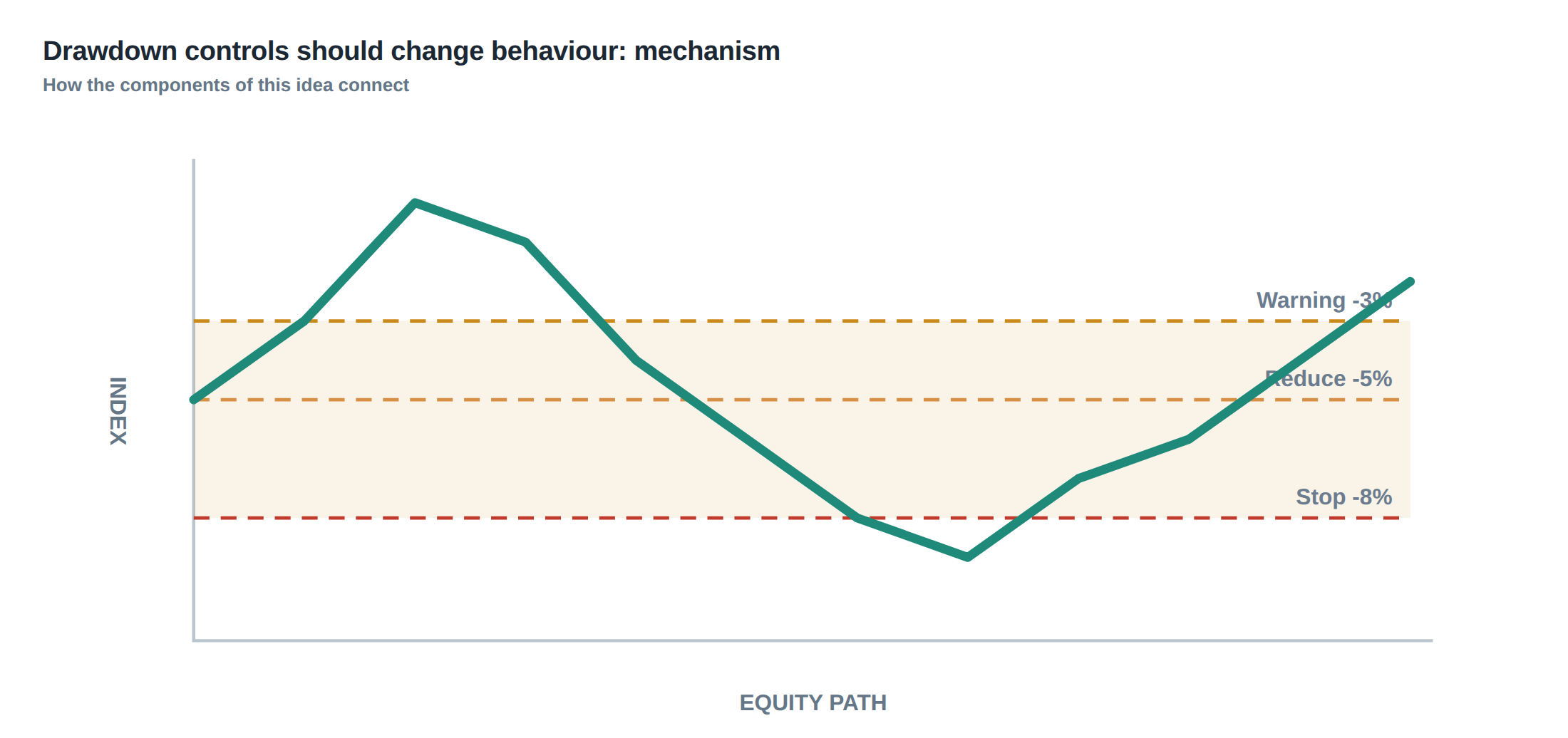
The first step is to define the measurement horizon. For each strategy we compute the peak‑to‑trough loss as a percentage of the allocated capital, updating the peak whenever a new high water mark is reached. Simultaneously we maintain a portfolio‑wide peak‑to‑trough figure that aggregates the individual contributions, weighted by current exposure.

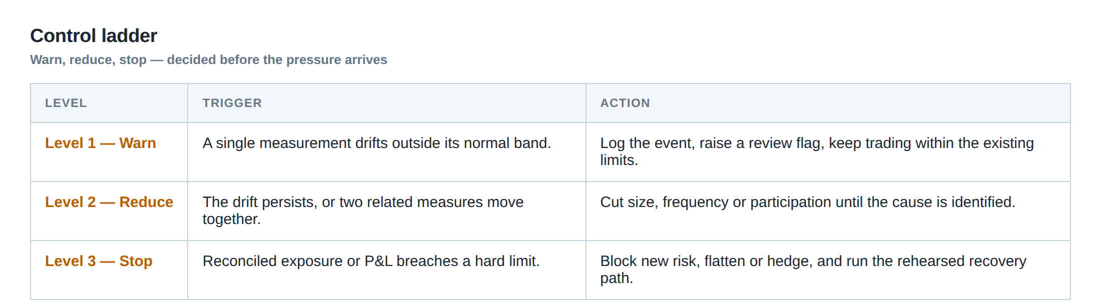
Second, we establish three quantitative thresholds: a warning level (typically 0.5 % of capital), a de‑risking level (1.0 % of capital), and a shutdown level (1.5 % of capital). Crossing the warning level triggers an automated alert and a mandatory review of recent execution statistics. Crossing the de‑risking level forces the system to halve the notional of the offending strategy and to pause any new position increases for a pre‑defined interval, often 30 minutes for high‑frequency signals. Crossing the shutdown level initiates a hard stop: the strategy is removed from the execution queue, its capital allocation is set to zero, and a post‑mortem is required before any re‑allocation is considered.

Third, the recovery path is governed by evidence. After a de‑risking event the algorithm must demonstrate that the loss distribution has returned to its baseline – for example, that the realised variance over the last 1 000 trades is within 10 % of the modelled variance, and that tail‑delay frequencies have dropped below a pre‑set percentile. Only when these statistical checks are satisfied can the system request a gradual restoration of risk, typically in 25 % increments, each gated by the same evidence criteria.

Finally, the framework records “time under water” – the duration for which the strategy remains below its previous peak. This metric is as important as the depth of the drawdown because prolonged exposure to reduced capital can erode optionality, limit the ability to capture favourable market moves, and increase the probability of hitting the shutdown threshold due to cumulative small losses.

A worked example with real numbers

Consider a medium‑frequency equity market‑making strategy that is allocated $20 million of capital. Its daily expected Sharpe ratio is 1.2, with a realised volatility of 1.5 % per day. The control parameters are set at 0.5 % (warning), 1.0 % (de‑risk), and 1.5 % (shutdown) of the allocated capital.

On Day 12 the strategy experiences a series of adverse fills caused by a sudden latency spike in the order‑routing gateway. The peak‑to‑trough loss reaches $210 000, which is 1.05 % of the allocated capital, thereby crossing the de‑risking threshold. The system automatically halves the notional exposure, reducing the daily gross notional from $150 million to $75 million. Simultaneously, the algorithm pauses any new position scaling for the next 45 minutes while it records the latency distribution.

During the subsequent 1 000 trades the realised variance falls to 1.4 % per day, still within the 10 % tolerance of the modelled 1.5 % target, but the 99th‑percentile latency has risen to 250 ms, above the acceptable 180 ms limit. Because the tail‑delay criterion is not satisfied, the system refuses to restore the original notional. Instead, it maintains the reduced exposure for an additional 24 hours while the routing issue is investigated.

By Day 14 the latency issue is resolved, the 99th‑percentile latency drops back to 160 ms, and the variance remains within tolerance. The system now permits a stepwise increase of exposure: first to 60 % of the original notional ($90 million), then after another 12 hours to 80 % ($120 million), provided the statistical checks continue to hold. The total time under water is 2 days, and the maximum depth of the drawdown was 1.05 %.

Contrast this with a naïve recovery approach where the trader, seeing the $210 000 loss, decides to double the position size the following day in order to “make the money back quickly”. The notional jumps to $300 million, exposing the strategy to a larger absolute loss if the latency spike persists. Within two days the loss escalates to $620 000, breaching the shutdown threshold of 1.5 % ($300 000). The system then forces a full shutdown, and the capital that could have been preserved under the disciplined de‑risking path is instead lost, illustrating how aggressive size increases can convert a recoverable model error into terminal ruin.

Where it breaks in live markets

Even the most meticulously designed drawdown controls can be undermined by market realities that are difficult to anticipate. One common failure mode is the correlation of multiple strategies to a hidden market factor – for example, a sudden shift in funding rates that simultaneously degrades the performance of several statistical arbitrage signals. If each strategy is monitored in isolation, the aggregate portfolio drawdown may climb unnoticed until the shutdown threshold is breached at the portfolio level, at which point the damage is already extensive.

Another breach occurs when the execution environment changes faster than the control parameters can be updated. A new exchange fee schedule, a change in tick size, or the introduction of a latency‑inducing firewall can alter the loss distribution in ways that are not captured by the historical variance or tail‑delay metrics. If the system continues to rely on stale statistical baselines, it may incorrectly deem the post‑event loss distribution to be “within tolerance”, allowing the strategy to remain fully exposed while the underlying risk has actually increased.

Human override is a subtle but potent source of failure. In a high‑pressure environment, a senior trader may be tempted to bypass the de‑risking rule, arguing that the market conditions are temporary. Without technical enforcement – for instance, a hard‑coded cap on position size that cannot be overridden without multi‑party approval – such discretionary actions can quickly erode the protective intent of the control framework.

Finally, the measurement of “time under water” can be ignored when the focus is solely on the depth of the drawdown. Prolonged periods of modest under‑performance can drain optionality, especially for strategies that rely on occasional large moves to achieve their expected return. If the control system does not penalise long durations below the peak, the trader may continue to allocate capital to a strategy that is no longer statistically viable, setting the stage for a later, larger drawdown.

The operating path, stage by stage

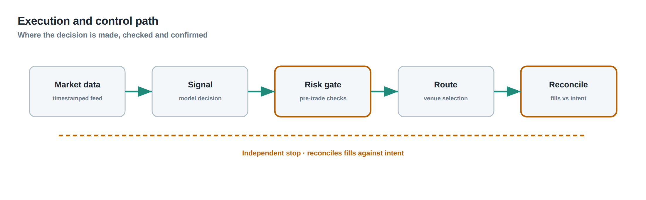
Stage 1 is the continuous monitoring loop. Every tick of the P&L engine updates the peak‑to‑trough loss for each strategy and for the portfolio, records the current latency distribution, and checks the realised variance against the modelled target.

Stage 2 is the threshold detection module. When a loss breaches a predefined percentage of allocated capital, the module raises a flag that is routed to the risk‑action engine. The flag contains the severity (warning, de‑risk, shutdown) and the identity of the affected strategy.

Stage 3 is the risk‑action engine. For a warning flag it sends a notification to the desk manager and logs the event. For a de‑risk flag it issues a command to the order‑management system to halve the notional, to suspend any scaling requests, and to start a timer that measures the time under water. For a shutdown flag it sends a hard stop command, sets the allocation to zero, and triggers a mandatory post‑mortem workflow that must be completed before any re‑allocation request can be submitted.

Stage 4 is the evidence‑gathering phase. While the strategy is de‑risked, the system collects a sample of recent trades, calculates the realised variance, and evaluates tail‑delay statistics. It also checks external signals such as market‑wide volatility indices to ensure that the environment has not deteriorated further.

Stage 5 is the recovery approval process. If the statistical evidence satisfies the pre‑defined tolerance bands, the system automatically proposes a stepwise restoration of risk. Each step is gated by a repeat of the evidence‑gathering phase. If the evidence fails, the system maintains the reduced exposure and may escalate to a shutdown if the loss deepens.

Stage 6 is the post‑mortem archiving. Once the strategy has either fully recovered or been permanently retired, the entire sequence of events – from the initial breach to the final outcome – is stored in a searchable database. This archive feeds into periodic reviews of the threshold settings and the statistical tolerances, ensuring that the control framework evolves with the market.

Controls that act before the damage

The most effective defence against catastrophic loss is to intervene before the drawdown reaches the de‑risking threshold. One class of pre‑emptive control is the “risk‑budget” monitor, which caps the daily variance contribution of each strategy to a fixed fraction of the total risk budget. When the realised variance of a strategy begins to drift upward, the monitor reduces the permissible notional in proportion, thereby limiting the potential loss before a breach occurs.

Another pre‑emptive measure is the “execution‑quality guardrail”. By continuously profiling latency, fill‑rate, and stale‑order frequency, the guardrail can detect a degradation in execution quality that historically precedes drawdowns. If the 95th‑percentile latency exceeds a threshold for more than five consecutive minutes, the guardrail automatically throttles the strategy’s order flow, effectively reducing exposure before the loss materialises.

A third safeguard is the “correlation‑stress test”. The system periodically injects a synthetic shock to the common factor exposures of all strategies – for example, a sudden widening of bid‑ask spreads – and observes the projected impact on the portfolio’s peak‑to‑trough loss. If the simulated loss exceeds a predefined safety margin, the system pre‑emptively reduces the allocation to the most sensitive strategies, thereby lowering the real‑world drawdown risk.

These controls are arranged in a ladder‑like hierarchy, with the most granular, strategy‑specific checks at the bottom and the broad, portfolio‑wide stress tests at the top. The ladder ensures that a breach at any level triggers the appropriate mitigation without waiting for the drawdown to become visible on the P&L screen.

How to measure whether it is working

Effectiveness is assessed by two complementary metrics: the frequency of threshold breaches and the average time under water after a breach. A well‑tuned control system should see a reduction in both over successive quarters. The first metric is straightforward – count the number of warning, de‑risk, and shutdown events per month and compare them to a baseline established before the controls were introduced.

The second metric, average time under water, captures the speed of recovery. By dividing the cumulative duration that each strategy spends below its previous peak by the number of breaches, we obtain a mean “recovery latency”. A falling recovery latency indicates that the evidence‑gathering and stepwise restoration processes are functioning as intended.

A third, more nuanced indicator is the “optional‑ity preservation ratio”. This is the proportion of the original capital that remains allocated to a strategy after a drawdown, adjusted for the expected return of the strategy over the recovery horizon. If the ratio stays above, say, 80 % for most strategies, it suggests that the controls are preserving the ability of the strategy to participate in favourable market moves, rather than forcing an early exit that would erode long‑term expectancy.

Finally, a qualitative audit of post‑mortem reports provides insight into whether the evidence thresholds are appropriately calibrated. If the majority of post‑mortems conclude that the statistical checks were either too lax or too strict, the thresholds should be adjusted. This feedback loop is essential for keeping the control framework aligned with evolving market dynamics.

The portfolio view

At the portfolio level the drawdown control framework must reconcile the individual strategy signals with the aggregate risk appetite. The portfolio peak‑to‑trough loss is computed by aggregating the weighted contributions of each strategy, taking into account their current notional, correlation, and the realised variance of the combined position.

When the portfolio‑wide loss breaches the warning level, the system issues a desk‑wide alert, prompting a review of the correlation matrix. If the de‑risking level is crossed, the portfolio manager is required to re‑balance the allocations, often by scaling down the most volatile or most correlated strategies first. This re‑balancing is performed automatically by a “risk‑budget optimiser” that solves a constrained minimisation problem: minimise the projected variance subject to the constraint that the total capital utilisation remains above a minimum threshold, typically 60 % of the allocated capital.

If the shutdown threshold is reached, the portfolio engine enforces a hard stop on the entire desk, liquidating positions in a risk‑aware order that prioritises the most liquid instruments to avoid market impact. The shutdown is only lifted after a full portfolio‑wide post‑mortem, which includes a review of the systemic factors that caused the drawdown – for example, a sudden liquidity crunch across multiple venues.

By maintaining a continuous view of both depth and duration of drawdowns at the portfolio level, the desk can preserve optionality for the strategies that remain statistically sound, while protecting the capital base from cascading failures. The interplay between strategy‑level controls and portfolio‑level re‑balancing creates a resilient architecture where a single adverse event is unlikely to cascade into a desk‑wide catastrophe.

Do you currently have a formal, evidence‑driven recovery path that must be demonstrated before you are allowed to restore full risk after a drawdown?

About the research behind this lesson

Andrew Lo's lectures build risk analysis from return distributions and statistical measures, rather than treating one realised result as a complete description of risk.

Applied to this lesson: For a fast strategy, median latency or average fill quality is not enough. The review has to include tail delays, stale-order frequency and the loss distribution when cancellation or routing behaves abnormally.

Explore PULSE: System details

PULSE live account: Verify the live account on FX Blue

Live chat and updates: Telegram @xtrskhft

Source: Risk and Return

Educational content only. Trading leveraged products involves risk.