October 15, 2026

What this problem really is

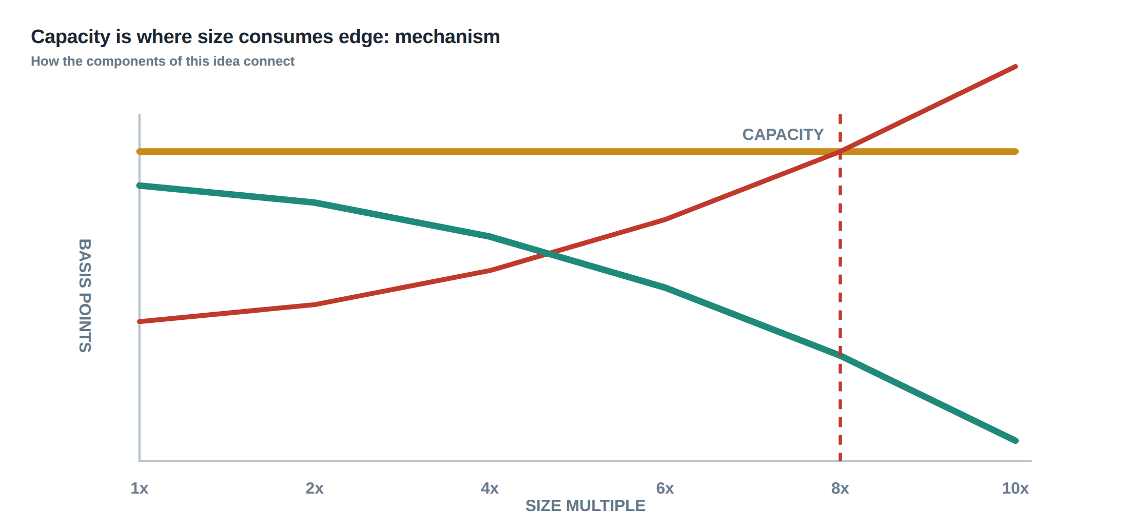
The term capacity in quantitative trading refers to the maximum notional that a strategy can deploy before its own execution costs erode the theoretical edge. In a perfectly liquid market the cost of buying or selling a given quantity would be independent of size; in reality each additional contract pushes the limit order book, widens the effective spread and leaves a permanent imprint on the price. When a model is calibrated on a few hundred contracts per day it may predict a Sharpe ratio of 2.5, yet the same model run on a few million contracts can become flat or even negative because the realised execution cost exceeds the expected gross alpha. The problem is therefore not a lack of predictive power but a mismatch between the statistical edge and the market’s ability to absorb the required turnover without moving the price against the trader.

How the mechanism works, step by step

Electronic markets operate as price‑time‑priority queues. An incoming limit order is placed behind all existing orders at the same price, and each trade removes the head of the queue. The value of a queue position can be split into three components. First, the spread capture earned by being at the best bid or offer; second, the adverse‑selection cost incurred when the next market order arrives from the opposite side; third, the option value of staying in line – the right to continue capturing the spread if the queue is not depleted.

When a strategy scales, the queue position it can afford to hold shrinks. A larger order must either increase its participation rate – the fraction of total volume it consumes – or accept a lower priority in the queue. Raising participation deepens the order into the book, exposing the trader to higher temporary impact: the immediate price concession required to execute the extra volume. Once the trade is completed, a permanent impact remains as the market updates its reference price to reflect the new supply‑demand balance. Finally, if the trader cannot finish the order before the price moves unfavourably, an opportunity cost is incurred because the expected spread capture is lost.

The interaction of these elements can be expressed compactly:

\[ \text{Total cost}= \underbrace{\text{Spread capture}}{\text{positive}}-\underbrace{\text{Temporary impact}}{\text{negative}}-\underbrace{\text{Permanent impact}}{\text{negative}}-\underbrace{\text{Opportunity cost}}{\text{negative}} . \]

When the sum turns negative the strategy has exhausted its capacity.

A worked example with real numbers

Consider a mean‑reversion micro‑structure model that trades a single stock with an average daily volume of 20 million shares and a realised volatility of 0.8 % (annualised ≈ 12 %). The model predicts a per‑share gross edge of 0.12 % of price, derived from capturing half a tick (0.5 bps) of spread on each round‑trip.

At a modest participation rate of 2 % the trader sends a 400 000‑share order split evenly between buy and sell legs. The temporary impact function is calibrated as

\[ \Delta p_{\text{temp}} = \kappa \left(\frac{Q}{V}\right)^{\beta}, \]

with \(\kappa = 0.03\) bps and \(\beta = 0.5\). Substituting \(Q=200\,000\) (per leg) and \(V=20\,000\,000\) gives a temporary impact of 0.03 × (0.01)^{0.5}=0.0095 bps per leg, negligible relative to the 0.5 bps spread capture. Permanent impact is modelled as 0.02 bps per 1 % of daily volume, therefore 0.04 bps for the 2 % participation. Opportunity cost is assumed to be 0.01 bps per minute of queue waiting; the average queue time at 2 % participation is 30 seconds, yielding 0.005 bps.

Net expected edge per share is therefore

\[ 0.5\text{ bps} – 0.0095\text{ bps} – 0.04\text{ bps} – 0.005\text{ bps}=0.4455\text{ bps}. \]

Now double the order size to a 800 000‑share participation of 4 %. The temporary impact becomes 0.03 × (0.02)^{0.5}=0.0134 bps per leg, a modest rise, but the order now has to walk down two price levels in the book to fill, exposing it to a price‑level depth of 2 ticks beyond the best price. Each extra tick costs an additional 0.5 bps, so the effective temporary impact is 0.0134 + 0.5 = 0.5134 bps. Permanent impact doubles to 0.08 bps, and the average queue time lengthens to 90 seconds, raising opportunity cost to 0.015 bps.

The net edge collapses to

\[ 0.5\text{ bps} – 0.5134\text{ bps} – 0.08\text{ bps} – 0.015\text{ bps}= -0.1084\text{ bps}, \]

a negative expectation despite the same underlying alpha. The example illustrates how a linear increase in notional can generate a super‑linear rise in execution cost when the order must penetrate deeper price levels, confirming that capacity is reached well before the theoretical edge disappears.

Where it breaks in live markets

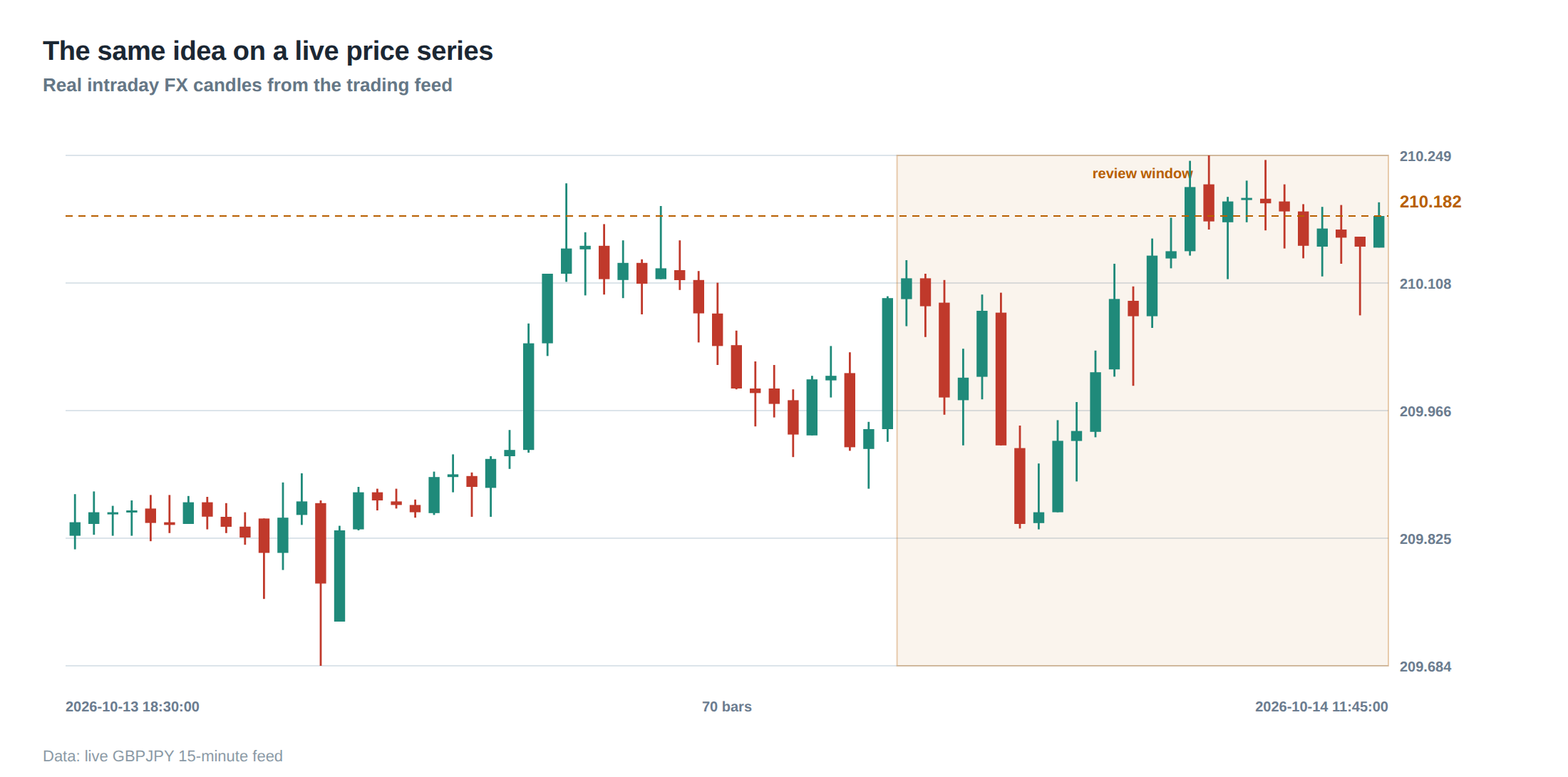
In practice the capacity ceiling is most frequently breached during thin‑liquidity sessions – for example, the first hour after a market opens, the last hour before close, or during macro‑event windows when order flow concentrates on a few symbols. In those periods the order book depth contracts, the spread widens and the probability of an urgent exit rises sharply. An algorithm that would normally sit patiently for a 30‑second queue may be forced to cross the spread to avoid a larger adverse‑selection loss when a news headline moves the reference price by several ticks.

The research on electronic markets treats the queue as a composite of spread capture, adverse‑selection risk and the option value of remaining in line. The implication is that the decision to keep an order alive cannot be based on elapsed time alone; the system must continuously reassess whether the remaining spread, adjusted for the increased adverse‑selection probability, still outweighs the cost of staying in the queue. When the market thins, the adverse‑selection component spikes, the option value collapses, and the optimal policy is to cancel or reduce the order rather than to persist.

The operating path, stage by stage

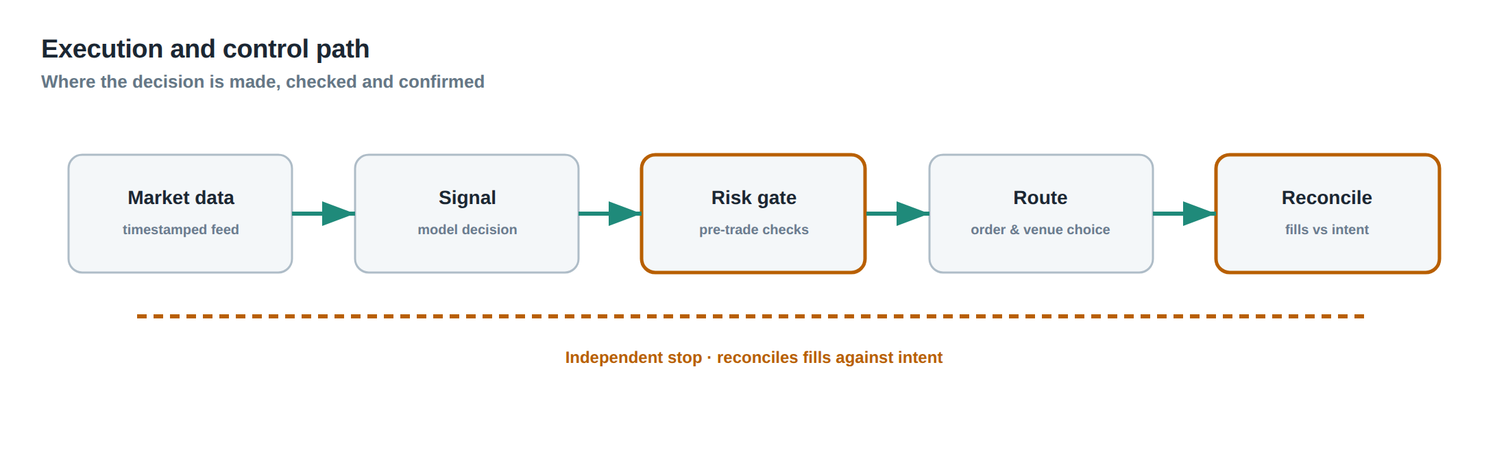
A robust capacity‑management workflow proceeds through a series of stages. First, the strategy’s theoretical edge is quantified on a per‑share basis using back‑tested signal‑to‑price relationships. Second, a capacity model translates that edge into a maximum participation rate by incorporating calibrated temporary and permanent impact functions, as well as an estimate of opportunity cost derived from historical queue times. Third, a simulation engine runs the strategy at incremental notional levels, measuring expected net edge at each step until the curve flattens to zero – this is the capacity curve. Fourth, the live order‑router uses the capacity curve to set an upper bound on order size for each execution window, adjusting dynamically for real‑time volatility and volume. Finally, a monitoring layer records realised slippage and compares it to the predicted cost at the corresponding participation rate; deviations trigger an automatic reduction in allowed size.

The flow of information is cyclical: each trading day feeds new realised cost data back into the impact calibrations, which in turn shift the capacity curve for the next iteration. The system therefore evolves with market conditions rather than relying on a static, one‑off estimate.

Controls that act before the damage

Pre‑trade controls act as the first line of defence against capacity overruns. A participation‑rate limiter checks the intended order size against the current daily volume estimate; if the ratio exceeds the calibrated ceiling, the order is sliced into smaller child orders. A volatility filter raises the impact coefficients when realised volatility spikes, effectively shrinking the permissible participation. A liquidity‑heat map monitors order‑book depth at the target price level; if depth falls below a multiple of the intended quantity, the algorithm either postpones execution or switches to a marketable order with a tighter time horizon.

A queue‑position estimator evaluates the expected waiting time based on current order‑book imbalance and recent fill rates. When the estimated wait exceeds a threshold that would make the option value of staying in line negative, the order is withdrawn. These controls operate before any capital is at risk, ensuring that the strategy never attempts to push more volume than the market can absorb without destroying its own edge.

How to measure whether it is working

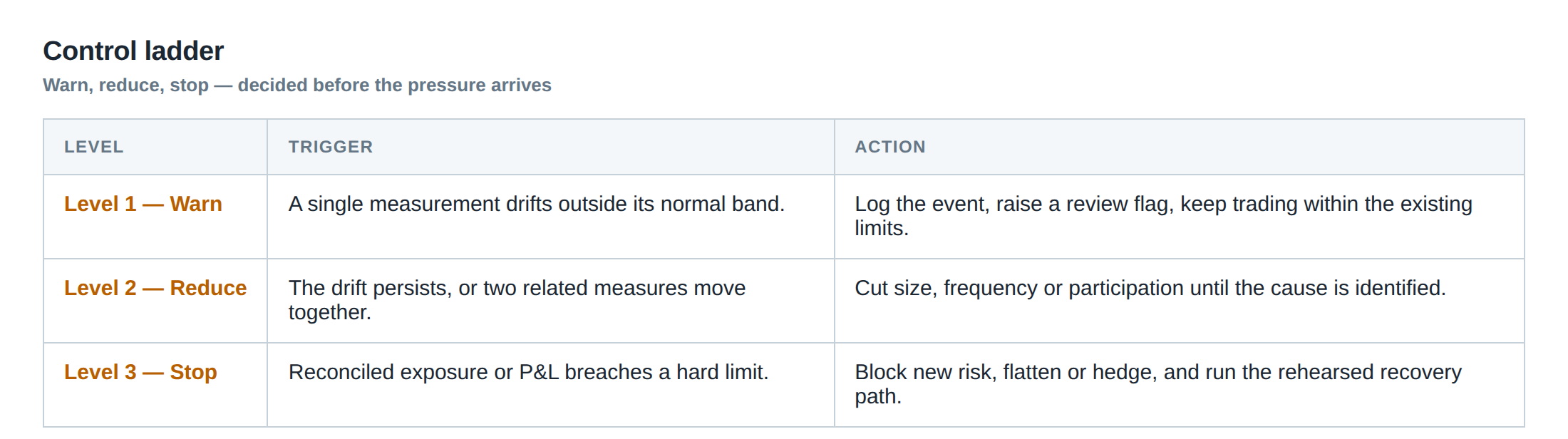
The primary metric is net realised edge per share, calculated as gross alpha minus all measured execution costs. To isolate the capacity effect, the edge is plotted against participation rate for each trading day; the resulting scatter should trace the pre‑computed capacity curve. Deviations are quantified by the slippage‑to‑capacity ratio: realised slippage divided by the modelled cost at the observed participation. A ratio consistently above one indicates that the impact model underestimates true market friction, prompting a recalibration.

Secondary diagnostics include the temporary‑impact coefficient derived from the linear regression of price move versus order size, and the permanent‑impact decay measured by the price path after the trade has completed. Opportunity cost can be inferred from the proportion of orders that were cancelled before full execution and the corresponding foregone spread capture. By aggregating these statistics across symbols, time‑of‑day buckets and volatility regimes, the desk can confirm whether the capacity controls are preserving edge across the full spectrum of market conditions.

The portfolio view

From a portfolio perspective capacity is a constraint that shapes allocation, risk budgeting and turnover limits. Each strategy contributes a capacity‑adjusted expected return, which is the product of its theoretical edge and the feasible participation rate after accounting for market frictions. When the aggregate desired turnover exceeds the total market capacity, the optimisation engine must re‑weight strategies, perhaps favouring those with higher edge‑to‑impact ratios or those that trade in less correlated instruments.

Because capacity is not static, the portfolio manager must monitor the capacity utilisation metric – the ratio of actual daily turnover to the sum of individual strategy capacity limits. A utilisation above 80 % signals that the desk is operating near the edge of market absorption and that any further scaling will likely erode performance. Conversely, a low utilisation suggests that additional capital could be deployed without compromising edge, provided the impact models are updated to reflect the new scale.

The portfolio view also integrates stress testing: scenarios such as a 30 % drop in liquidity during a macro shock, or a sudden widening of spreads by 100 bps, are simulated to verify that the capacity curve retains a positive net edge under extreme conditions. The outcome informs the setting of risk‑adjusted capacity buffers that keep the desk comfortably inside the safe operating region.

In practice, the continuous feedback loop between realised slippage, impact model recalibration and capacity‑adjusted allocation is what separates a desk that can grow its strategies sustainably from one that sees its edge evaporate as soon as it attempts to scale.

Will the next increment of capital you allocate survive the market’s own resistance, or will it simply be absorbed as cost?

About the research behind this lesson

The seminar frames electronic markets as price-time-priority queues. It separates queue value into spread capture versus adverse-selection cost and the option value of retaining a place in line.

Applied to this lesson: An order lifetime therefore cannot be based on elapsed time alone: the system must reassess whether its queue position, expected spread and adverse-selection risk still justify keeping the order alive.

Explore PULSE: System details

PULSE live account: Verify the live account on FX Blue

Live chat and updates: Telegram @xtrskhft

Source: High-Frequency Trading and Modern Market Microstructure

Educational content only. Trading leveraged products involves risk.