October 14, 2026

What this problem really is

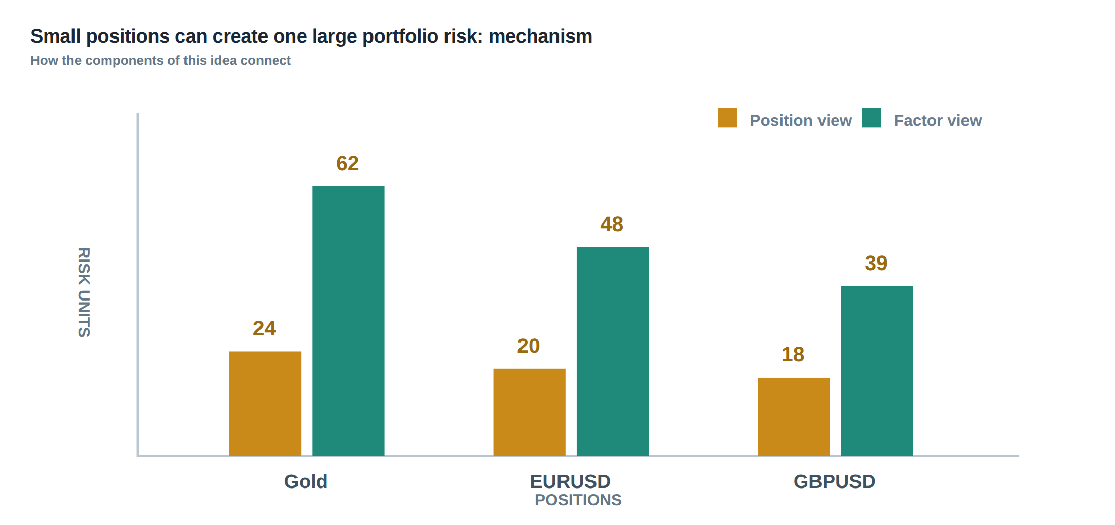
The risk that a portfolio appears safe when each position is examined in isolation is a classic illusion. Individual limits – a 2 % cap on delta, a 1 % cap on beta, a 5 % cap on currency exposure – are useful for preventing a single trade from blowing up the book, but they do not capture the hidden web of common drivers that bind seemingly unrelated positions together. When five modest long contracts all depend on the same “risk‑on” dollar factor, their aggregate delta, beta and volatility exposure can equal that of a single highly‑leveraged trade. The problem is not the size of any one order; it is the aggregation of factor sensitivities that is invisible to per‑trade checks.

The phenomenon becomes acute in multi‑asset desks where equities, futures, FX forwards and credit spreads are all priced off a shared set of macro variables. A modest uptick in the US dollar index can simultaneously erode the expected return of a European equity index future, a commodity‑linked ETF, a high‑yield bond spread and a carry trade. If each instrument is limited to a 0.5 % dollar exposure, the combined effect may be a 2.5 % exposure that is well beyond the desk’s risk appetite. In practice, the loss distribution of the portfolio develops a heavy tail, even though each leg looks benign in calm‑period back‑tests.

The core thesis, therefore, is that limits set at the trade level miss the common factors and correlations that connect positions across markets. A portfolio risk framework must start from the aggregate factor view, not from the sum of independent caps. Only then can a desk anticipate the “one large portfolio risk” that small positions collectively create.

How the mechanism works, step by step

First, each trade is decomposed into its factor loadings: delta to the underlying price, beta to a market index, currency exposure, duration for fixed‑income legs, and sensitivity to volatility regimes. This decomposition is typically performed with a linear regression or a principal‑component analysis on a rolling window of returns. The resulting factor vector is stored alongside the trade’s notional.

Second, the desk aggregates the factor vectors across all open positions. The sum of the delta components yields the portfolio‑wide directional exposure; the sum of the beta components gives the market‑wide systematic exposure; the sum of the currency components shows net foreign‑exchange risk; the sum of duration components reflects interest‑rate sensitivity; and the sum of volatility‑factor exposures indicates how the portfolio will behave when implied volatilities shift. At this stage, the desk can also calculate cross‑factor covariances, for example how a move in the dollar index correlates with a change in equity volatility.

Third, the aggregated exposures are compared to pre‑defined stress thresholds rather than to the calm‑period limits used for individual trades. Stress thresholds are derived from scenario analysis – a 5 % move in the dollar, a 200‑basis‑point swing in the 10‑year yield, a 30 % jump in VIX – and represent the maximum tolerable loss under those conditions. If the summed exposure exceeds any stress threshold, the system flags a concentration risk even though no single trade violates its own cap.

Finally, the desk decides whether to unwind, hedge or rebalance. Because the risk is factor‑driven, the corrective action often involves a small number of offsetting trades that neutralise the offending factor, rather than closing each individual position. This approach preserves alpha while restoring the portfolio to a safe factor profile.

A worked example with real numbers

Consider a desk that holds five long futures contracts, each with a notional of USD 10 million: an S&P 500 e‑mini, a Euro‑Stoxx 50, a crude‑oil calendar spread, a US‑Treasury 10‑year note, and a high‑yield corporate bond index future. The individual limits are set at 2 % delta, 1 % beta to the global equity index, and 0.5 % exposure to the US dollar. On paper each contract sits comfortably within those caps.

When the factor decomposition is performed, the following sensitivities emerge (all expressed as a percentage of the contract notional):

S&P 500: delta +1.2 %, beta +0.9 %, dollar +0.3 % Euro‑Stoxx 50: delta +1.1 %, beta +0.8 %, dollar +0.4 % Crude‑oil spread: delta +0.9 %, beta +0.2 %, dollar +0.5 % 10‑year Treasury: delta +0.6 %, beta +0.1 %, dollar +0.2 % * High‑yield bond: delta +1.0 %, beta +0.7 %, dollar +0.4 %

Summing across the five contracts gives an aggregate delta of +4.8 %, an aggregate beta of +3.7 % to the global equity factor, and a combined dollar exposure of +1.8 %. The delta alone is more than double the per‑trade limit, and the beta is nearly four times the individual cap. In a stress scenario where the US dollar falls 5 % against a basket of currencies, the dollar‑sensitive component of the portfolio would lose roughly 1.8 % × 5 % ≈ 9 % of its notional – a loss comparable to a highly levered position.

If the desk were to ignore the factor aggregation and rely solely on the per‑trade caps, it would be blindsided by a single market move that simultaneously hits all five positions. The example demonstrates how modest, diversified‑looking trades can behave like one large, levered bet when they share a common driver.

Where it breaks in live markets

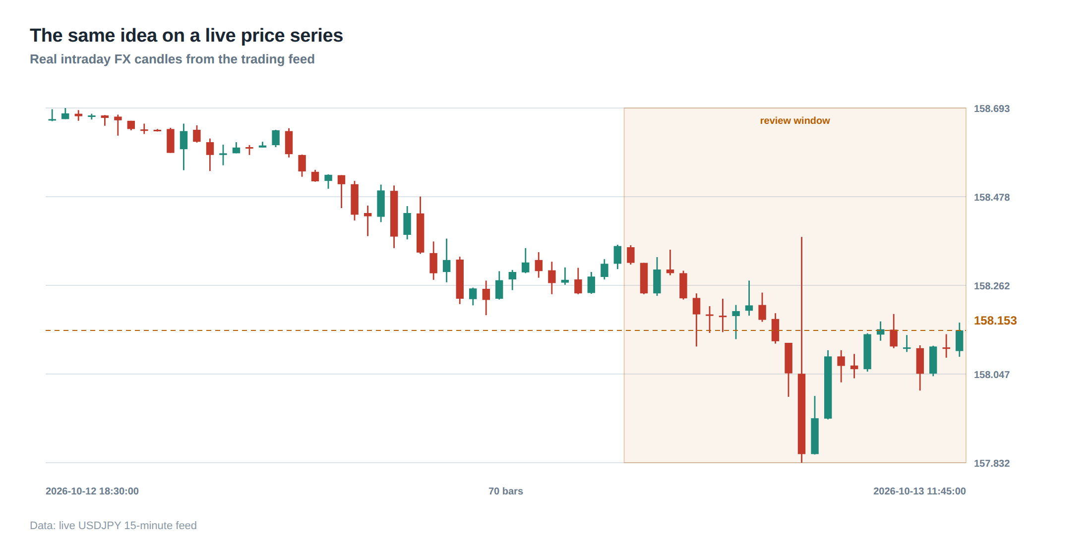
The theoretical aggregation described above assumes that factor loadings are stable and that correlations observed in historical data persist. In reality, market regimes shift, liquidity dries up, and financing costs change abruptly. During a rapid risk‑off episode, the dollar often strengthens, equity betas surge, and implied volatilities spike, causing the factor sensitivities to move in the same direction as the market shock. The desk’s stress thresholds, calibrated on calm‑period data, become under‑estimates of the true exposure.

Liquidity can also collapse on the very instruments that provide the hedge. If the desk attempts to neutralise its dollar exposure by selling short a USD‑indexed futures contract, the order book may be thin, leading to a large price impact and widening spreads. The resulting execution slippage adds to the loss, turning a modest 1.8 % dollar exposure into a far larger realised loss. Moreover, financing dependencies – such as the need to roll over short‑dated futures or to fund carry trades – can create a second‑order contagion. When funding rates spike, the cost of holding the same positions rises, eroding the profit margin and potentially triggering margin calls.

The combination of regime‑dependent factor shifts, liquidity crunches and financing stress creates a feedback loop. The desk’s risk models, which rely on static covariance matrices, fail to capture the dynamic amplification, and the portfolio can move from a “safe” state to a critical one within a few trading sessions.

The operating path, stage by stage

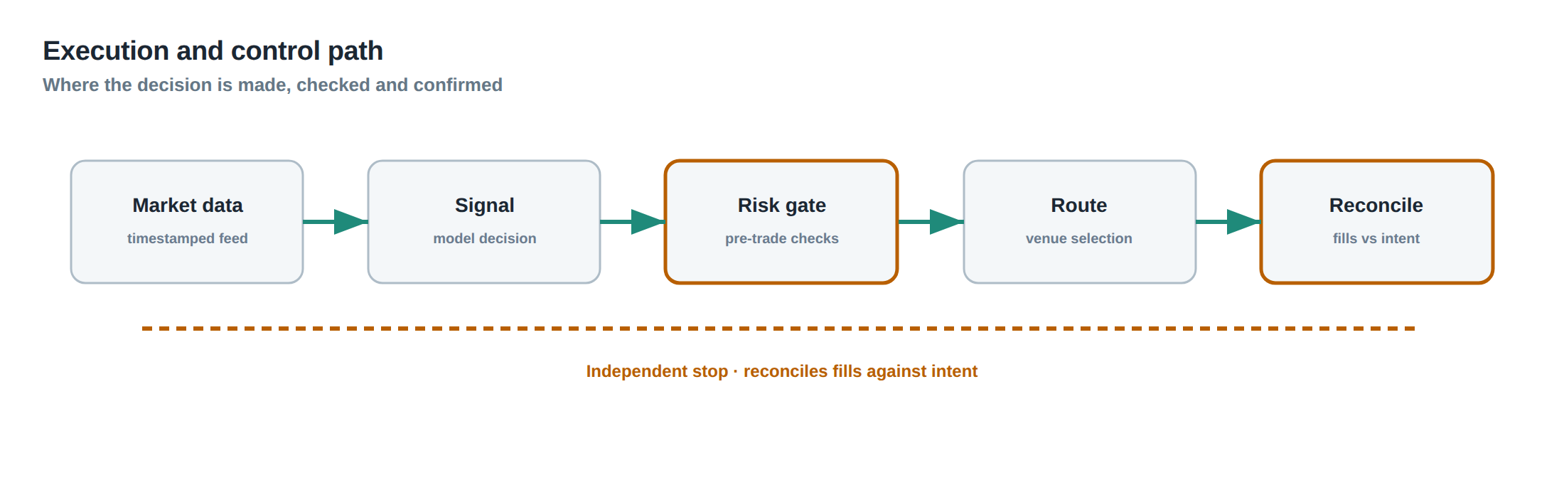
The first stage is data ingestion. Market data feeds, trade blotters and financing curves are collected in real time and stored in a time‑series database. The second stage is factor extraction, where each new trade is automatically decomposed into its delta, beta, currency, duration and volatility‑factor components using the latest regression coefficients. The third stage is aggregation, where the system sums the factor vectors across the entire open‑interest set and updates the portfolio‑wide exposure metrics.

The fourth stage is scenario testing. Pre‑defined stress scenarios – for example a 5 % dollar depreciation, a 300‑basis‑point rise in 10‑year yields, a 40 % jump in VIX – are applied to the aggregated factor exposures to generate a hypothetical loss distribution. The fifth stage is limit checking, where the projected losses are compared against the desk’s concentration thresholds for each factor. If any threshold is breached, an alert is raised and a workflow is triggered.

The final stage is remediation. The workflow presents the offending factor, the magnitude of the breach, and a list of possible offsetting trades. Traders can then execute a hedge, reduce notional, or rebalance the portfolio. Throughout, audit logs capture the decision path, providing a trail for post‑mortem analysis.

Controls that act before the damage

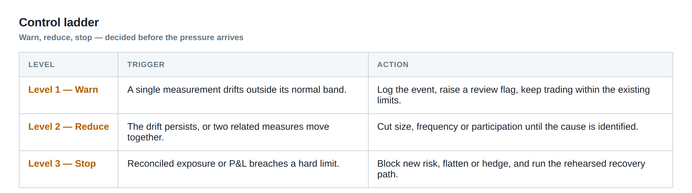
A robust control framework begins with pre‑trade validation. When a trader submits a new order, the system instantly projects the post‑trade factor exposure and aborts the order if the resulting aggregate delta, beta or currency exposure would exceed the stress limits. This “gate‑keeping” rule prevents the gradual build‑up of hidden concentrations.

Second, the desk should implement a factor‑level stop‑loss that automatically reduces exposure when a factor moves beyond a certain threshold in real time. For example, if the dollar index drops 2 % within an hour, the system can trigger a partial unwind of all dollar‑long positions, irrespective of the individual trade’s performance. This dynamic response curtails the tail risk that only materialises during extreme moves.

Third, financing‑risk buffers are required. By maintaining a cushion of high‑quality collateral and by diversifying funding sources, the desk reduces the chance that a spike in repo rates forces a rapid deleveraging of the whole book. The buffer is measured as a percentage of the net notional and is reviewed weekly.

Finally, regular stress‑testing cycles that incorporate “reverse‑stress” scenarios – where the assumed factor correlation matrix is inverted – help to uncover hidden dependencies that are not evident in historical data. The results feed back into the limit‑setting process, tightening thresholds where necessary.

How to measure whether it is working

The primary metric is the gap between the portfolio’s realised loss distribution and the loss distribution predicted by the aggregated factor model under stress. A narrowing gap over successive months indicates that the factor‑level controls are aligning the realised risk with the modelled risk. Secondary metrics include the frequency of factor‑limit breaches, the average time to remediate a breach, and the proportion of trades that are rejected at the pre‑trade gate.

Another useful gauge is the “factor‑concentration ratio”, defined as the aggregate exposure to a single factor divided by the total absolute exposure across all factors. A ratio consistently below 20 % suggests a well‑diversified factor profile. Conversely, a rising ratio signals that the desk is unintentionally re‑concentrating risk, prompting a review of the underlying trade ideas.

Finally, the desk should monitor the tail of the execution‑delay distribution for each venue. In fast‑moving markets, median latency is insufficient; the 99.9th‑percentile delay and the incidence of stale orders become leading indicators of liquidity‑related risk that can exacerbate factor exposures. By tracking these operational metrics alongside the factor exposures, the desk can assess whether the control stack is effective in real time.

The portfolio view

From the portfolio perspective, risk is no longer a collection of independent trade‑level caps but a multidimensional surface defined by factor exposures, liquidity constraints and financing dependencies. The aggregate delta tells us how much the portfolio will move with the underlying market; the aggregate beta reveals the systematic pull from global indices; the currency and duration components show the sensitivity to macro‑economic shifts; and the volatility‑factor exposure captures the convexity to market stress.

When these dimensions are mapped onto shared liquidity pools – for example, the same USD funding curve that supports both equity futures and carry trades – the portfolio inherits a common source of fragility. Stress testing that respects the joint distribution of these factors, rather than treating each in isolation, yields a more realistic picture of the tail risk. By limiting concentration at the factor and scenario level, the desk can maintain a diversified return stream while protecting against the hidden amplification that small, correlated positions can generate.

Do you currently aggregate factor exposures across all desks, or do you still rely on per‑trade limits to safeguard your portfolio?

About the research behind this lesson

Andrew Lo's lectures build risk analysis from return distributions and statistical measures, rather than treating one realised result as a complete description of risk.

Applied to this lesson: For a fast strategy, median latency or average fill quality is not enough. The review has to include tail delays, stale-order frequency and the loss distribution when cancellation or routing behaves abnormally.

Explore PULSE: System details

PULSE live account: Verify the live account on FX Blue

Live chat and updates: Telegram @xtrskhft

Source: Risk and Return

Educational content only. Trading leveraged products involves risk.