October 15, 2026

What this problem really is

In electronic markets the most visible metric of an execution algorithm is the fill‑rate: the proportion of submitted orders that eventually trade. A high fill‑rate is usually taken as a badge of reliability, suggesting that the algorithm is good at “getting in the market”. The reality is more nuanced. When a large share of fills occurs while the market is still moving favourably, the apparent success can be illusory. The true test is whether the realised profit after each fill survives the next price movement. If the order queue is constantly replenished just before the market reverses, the cumulative spread captured may be wiped out by a single adverse‑selection event. In that sense a passive fill can be bad news – the fill itself is not the problem, the timing relative to price dynamics is.

The underlying cause is that order lifetime is often judged by wall‑clock time alone. Traders assume that an order that has been alive for, say, 500 ms is still “in the queue” and therefore still valuable. Yet the value of a queue position decays as the expected future spread narrows and the probability of an adverse price move rises. The queue therefore carries two components of value: the expected spread capture (the “price‑time” component) and the option value of remaining in line (the “waiting” component). When the latter evaporates, a fill that looks benign on the surface may actually be a loss.

The problem is amplified in markets where the order book is thin or where latency‑sensitive participants dominate. A passive order that sits at the top of the book may be filled repeatedly as the market drifts, only to be hit by a large market‑order sweep that pushes the price away from the filled level. The trader records a series of small, positive P&L ticks, but the net result after the sweep is negative. The high fill‑rate therefore masks a hidden execution cost – the cost of being in the queue when the market turns.

How the mechanism works, step by step

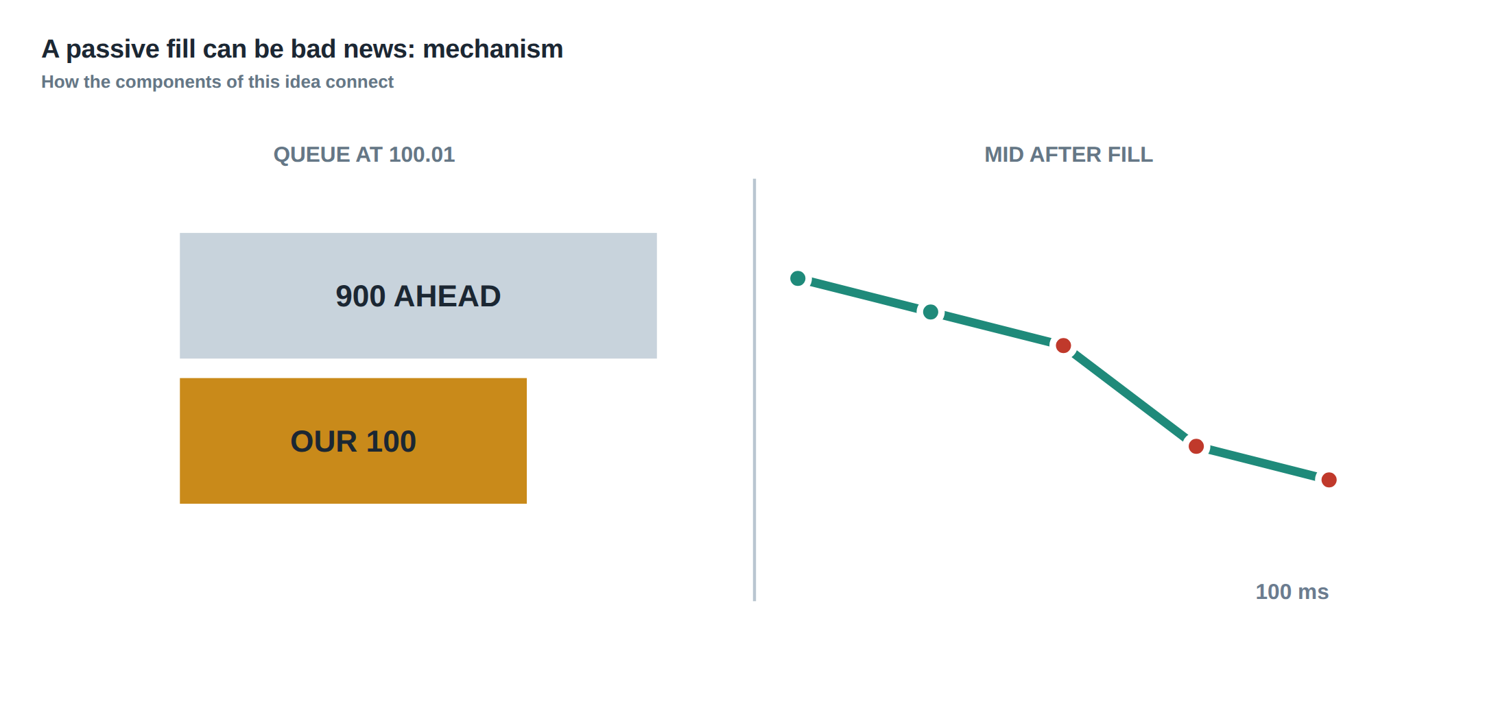
First, the algorithm estimates the expected volume that will arrive before the order is likely to be cancelled. This estimate uses recent trade intensity, order‑book depth, and the known latency of the gateway. The estimate is not static; it is updated on each market data tick, allowing the system to anticipate whether the remaining queue position is likely to be filled before the next price move.

Second, the algorithm monitors the mid‑price trajectory after each fill. The mid‑price is the arithmetic mean of the best bid and best ask at the moment the fill occurs. By recording the subsequent price path for a short horizon – typically a few hundred milliseconds to a few seconds – the system can compute the realised spread that the fill actually delivered. If the price drifts away, the realised spread shrinks, and the fill becomes a “toxic” event.

Third, the realised spread is compared with the quoted spread that was offered at the time of order entry. The quoted spread is the difference between the price at which the order sits and the opposite side of the book. The realised spread is the actual profit after the market moves, and it can be markedly lower, especially when the market moves against the order shortly after execution.

Fourth, the algorithm segments the data by market conditions – order‑book imbalance, realised volatility, and venue. Imbalance measures the relative depth on the bid versus the ask; volatility captures the magnitude of price changes over the measurement horizon; venue distinguishes between lit exchanges and dark pools. By stratifying the results, the system can identify under which circumstances passive fills become detrimental.

Finally, the algorithm contrasts “missed fills” – opportunities where the order was cancelled before a favourable move – with “toxic fills” – fills that were followed by an adverse price swing. The net effect of these two classes determines whether a high fill‑rate is genuinely beneficial or merely a façade.

A worked example with real numbers

Consider a small‑cap equity with a tick size of 0.01 £ and an average quoted spread of 0.04 £ (four ticks). An execution algorithm places a passive limit order at the best bid, aiming to capture the full spread. Over a ten‑second window the order is filled nine times, each time at the quoted price of 100.00 £ while the best ask sits at 100.04 £. The realised spread for each of those nine fills is therefore 0.04 £, giving a cumulative capture of 0.36 £ (nine × 0.04 £).

At the tenth attempt the order sits again at the best bid, but a large market sell order arrives a few milliseconds later, sweeping the book to 99.60 £. The passive order is filled just before the sweep, at 100.00 £, and the mid‑price immediately after the fill drops to 99.80 £. The realised spread on this single fill is therefore –0.20 £ (the price moved 0.20 £ against the order, equivalent to a loss of twenty ticks). The net P&L for the ten‑fill sequence becomes 0.36 £ – 0.20 £ = 0.16 £, a 55 % reduction from the naïve expectation that nine small gains would dominate.

If the algorithm had relied solely on the fill‑rate (10 / 10 = 100 %), it would have reported perfect execution. The realised spread analysis, however, reveals that a single toxic fill erased more than half the profit earned from the preceding nine benign fills. The example underscores why high fill‑rate alone cannot be taken as evidence of good execution.

Where it breaks in live markets

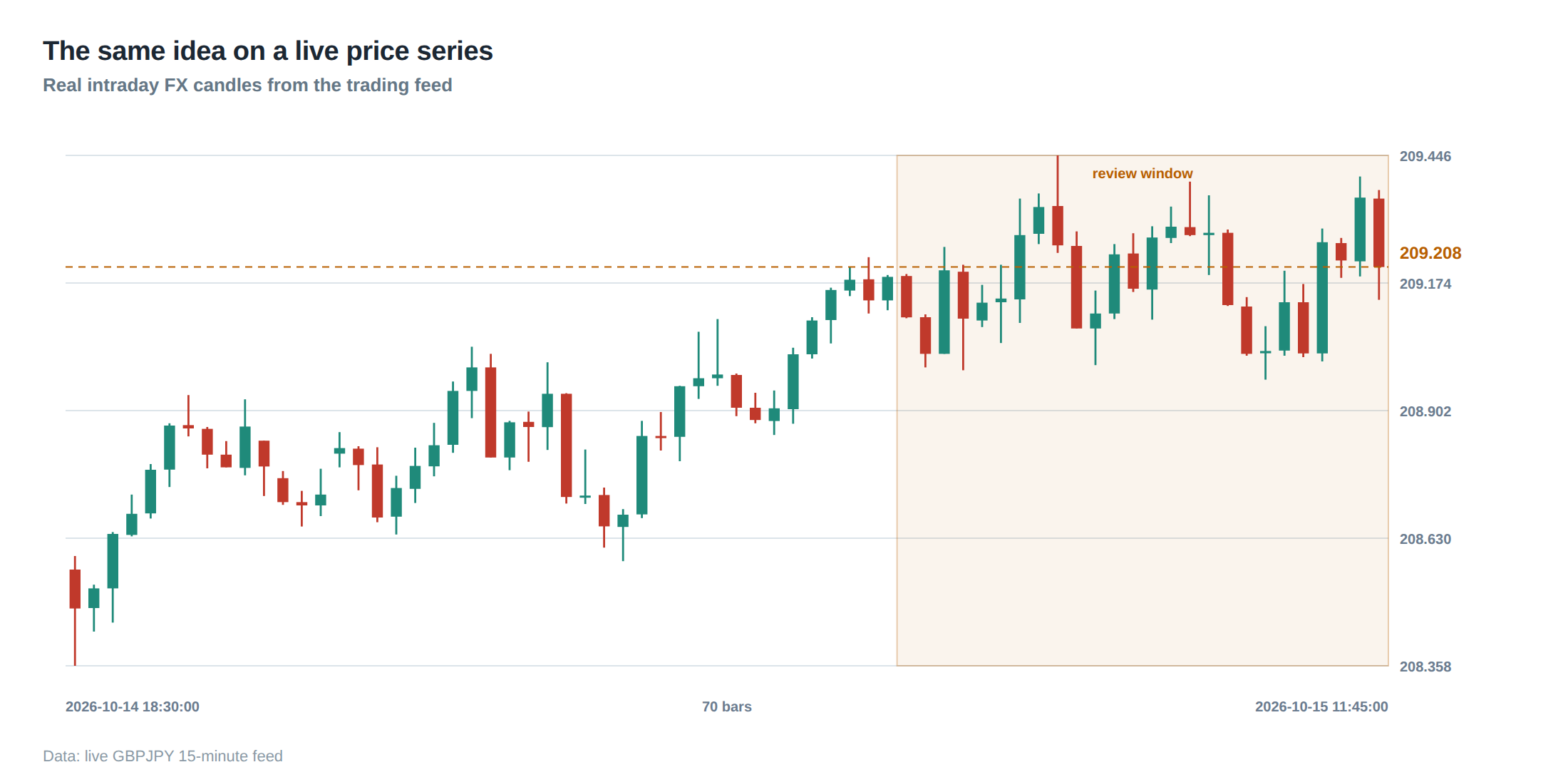
In live trading the idealised assumptions of the example are constantly challenged. Market depth can evaporate within a single heartbeat, and hidden liquidity may surface only after a price move. When order‑book imbalance becomes extreme – for instance, when the bid side holds only one lot while the ask side holds ten – the probability that a passive bid will be filled before a price drop rises sharply. The algorithm may still interpret the fill as a success, yet the subsequent price trajectory is more likely to be adverse.

Volatility spikes further destabilise the relationship between fill and realised spread. A sudden increase in realised volatility – measured, for example, by a three‑second realised variance that doubles – shortens the window in which a captured spread can be protected. The same passive order that would have earned a modest profit in a calm market can now be exposed to a rapid swing that turns the fill toxic.

Venue fragmentation adds another layer of risk. Some venues offer superior latency but lower depth, while others provide deep order books at the cost of slower execution. An algorithm that routes aggressively to the fastest venue may achieve a high fill‑rate, yet the fills may be concentrated in a thin book where a single aggressive market order can wipe out the accrued spread. Conversely, routing to a deep venue may lower the fill‑rate but improve the quality of each fill, reducing the incidence of toxic events.

The confluence of these factors means that the “fill‑rate = good execution” rule breaks down precisely when the market conditions that make a passive fill attractive also increase the likelihood of an adverse price move. The algorithm must therefore incorporate a dynamic risk assessment that looks beyond the binary fill/no‑fill outcome.

The operating path, stage by stage

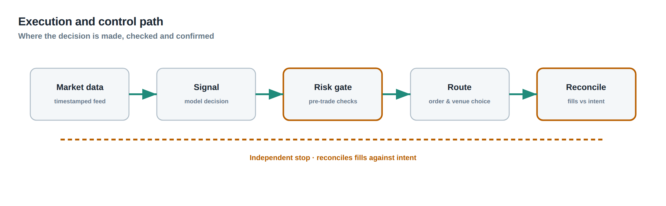
Stage one begins with the order‑generation module, which selects the target price, venue, and initial lifetime based on the current market snapshot. The module queries the latest order‑book imbalance, recent trade flow, and short‑term volatility estimate, then assigns a provisional queue‑value that reflects both expected spread capture and the option value of staying in line.

Stage two passes the order to the routing engine. Here the system evaluates the latency‑cost trade‑off across venues and chooses the path that maximises the expected queue‑value. The routing decision is not static; if the volatility estimate spikes during the routing latency, the engine can abort the transmission and re‑issue the order with a tighter price or a shorter lifetime.

Stage three is the monitoring loop. As soon as the order is on the book, a high‑frequency listener records every market‑data update, every fill, and every cancellation request. The loop computes the realised spread for each fill in real time, updating the cumulative P&L and the conditional probability that the next fill will be toxic. If the probability exceeds a pre‑set threshold, the loop triggers a protective action.

Stage four is the protective action module. It may cancel the order, amend the price, or shift the order to a different venue. The decision is driven by a cost‑benefit comparison: the expected loss from a potential toxic fill versus the expected gain from remaining in the queue. The module also logs the decision rationale for post‑trade analysis.

Stage five concludes with the post‑trade reconciliation process, where the realised spread data are aggregated, segmented by market condition, and stored in a performance database. The database feeds back into the order‑generation module, allowing the system to learn the conditions under which high fill‑rates become misleading.

Controls that act before the damage

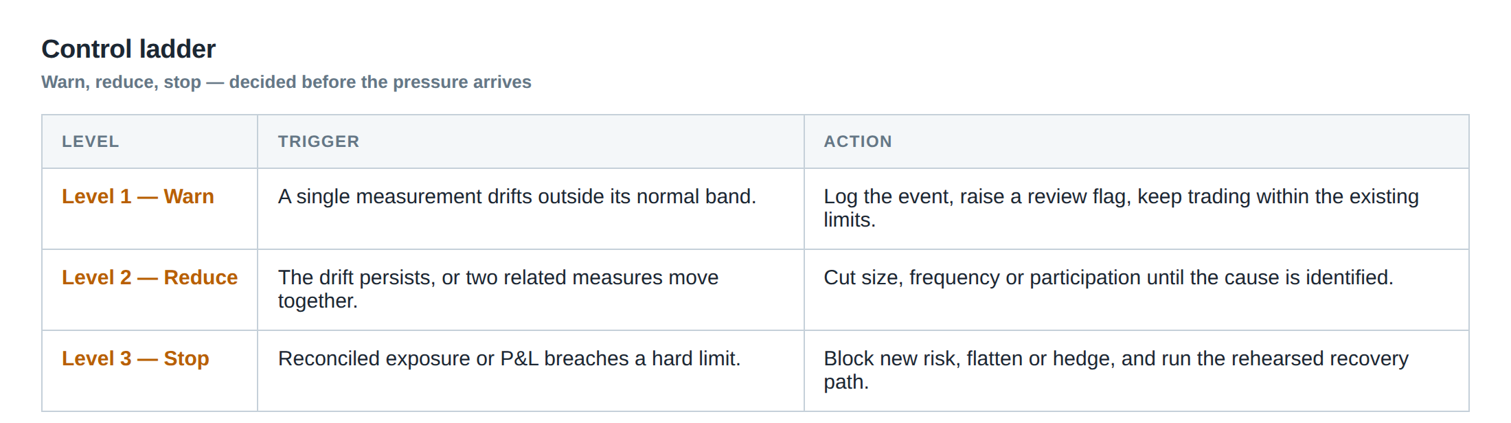
A robust control framework must intervene before a toxic fill can materialise. The first line of defence is a dynamic volume‑ahead estimator that projects how much liquidity will arrive before the order is likely to be cancelled. By comparing the projected volume with the size of the passive order, the system can decide whether to scale down the order size or to increase the aggressiveness of the price.

The second control monitors the rate of change of the mid‑price after each fill. If the mid‑price moves more than a predefined fraction of the quoted spread within a short horizon (for example, 0.5 % of price within 200 ms), the system flags the fill as potentially toxic and can instantly cancel any remaining passive exposure.

A third safeguard is the “realised‑spread filter”. It continuously computes the difference between quoted and realised spread for the most recent fills. When the realised spread falls below a certain proportion of the quoted spread – say, 30 % – the filter triggers a reduction in order lifetime or a shift to a more aggressive order type.

The fourth control stratifies exposure by market‑state buckets. By assigning each order a bucket based on current imbalance, volatility, and venue, the system can enforce stricter limits on fill‑rate expectations in high‑risk buckets. For instance, in a bucket where the bid‑ask imbalance exceeds 80 % and realised volatility is above the 75th percentile, the maximum allowed passive order size may be capped at 10 % of the nominal daily volume.

These controls operate in parallel, each feeding a risk score that must stay below a configurable threshold. When the composite score breaches the limit, the system automatically executes the protective action defined in the operating path, thereby preventing a cascade of toxic fills.

How to measure whether it is working

Measurement begins with the realised‑spread ratio, defined as the sum of realised spreads divided by the sum of quoted spreads for all fills in a given period. A ratio close to one indicates that most fills are capturing the expected spread; a ratio significantly below one signals that toxic fills are eroding performance. The ratio should be computed separately for each market‑state bucket to isolate conditions where the controls are most needed.

Second, the missed‑fill versus toxic‑fill differential provides insight into the trade‑off between aggressiveness and passivity. Missed fills are counted when an order is cancelled while the market is still moving favourably (mid‑price moving toward the order price). Toxic fills are counted when a fill is followed by an adverse price move that exceeds a pre‑defined threshold (for example, a move larger than two ticks within 300 ms). The net effect is the difference between the cumulative missed‑fill opportunity cost and the cumulative toxic‑fill loss.

Third, the average queue‑value decay time is a useful proxy for how quickly the option value of staying in line disappears under current market conditions. By measuring the time from order entry to the point where the expected realised spread falls below a target level, the desk can benchmark whether its lifetime settings are too generous.

Finally, a statistical test such as a paired t‑test between the realised‑spread ratios before and after a control adjustment can confirm whether the change has a significant impact. The test should be run on a rolling window to capture evolving market dynamics. Consistently positive test outcomes across multiple venues and volatility regimes validate that the controls are delivering the intended protection.

The portfolio view

When the analysis is extended from a single instrument to a portfolio, the impact of toxic fills becomes more pronounced. A single adverse event on a highly correlated asset can propagate through the risk‑budget, eroding the realised spread on other positions that are still in the queue. The portfolio‑level realised‑spread ratio therefore aggregates the individual ratios, weighted by each instrument’s exposure and by the correlation matrix.

Risk managers should monitor the portfolio’s exposure to “fill‑rate illusion” by tracking the aggregate toxic‑fill loss as a percentage of total spread captured. If that percentage climbs above a preset ceiling – for example, 20 % – the desk may need to tighten order‑lifetime parameters across the board or re‑allocate volume to more aggressive strategies.

Moreover, the portfolio view enables the identification of systemic patterns. If toxic fills cluster around specific times of day, news releases, or particular venues, the desk can adjust its routing preferences or temporarily suspend passive participation in those windows. Conversely, periods where the missed‑fill cost dominates may justify a more patient approach, allowing the algorithm to stay longer in the queue to harvest small spreads.

By treating fills as a portfolio of micro‑trades rather than isolated events, the desk gains a clearer picture of how high fill‑rates translate into true economic value. The ultimate metric is not the proportion of orders that fill, but the net realised spread after accounting for the hidden cost of toxic fills. When that metric is positive and stable across market regimes, the execution strategy can be deemed robust.

Do you currently assess the realised spread of each fill, or do you still rely mainly on fill‑rate as a performance indicator?

About the research behind this lesson

The seminar frames electronic markets as price-time-priority queues. It separates queue value into spread capture versus adverse-selection cost and the option value of retaining a place in line.

Applied to this lesson: An order lifetime therefore cannot be based on elapsed time alone: the system must reassess whether its queue position, expected spread and adverse-selection risk still justify keeping the order alive.

Explore PULSE: System details

PULSE live account: Verify the live account on FX Blue

Live chat and updates: Telegram @xtrskhft

Source: High-Frequency Trading and Modern Market Microstructure

Educational content only. Trading leveraged products involves risk.