October 10, 2026

⛶

What this problem really is

The temptation on a prop‑trading desk is to equate “speed” with “edge”. A sub‑millisecond improvement in order‑to‑exchange latency is celebrated, yet the underlying economics of a trade are rarely examined. In modern electronic markets every order is a claim on a position in a price‑time‑priority queue. The value of that claim is split between the portion that captures the quoted spread and the portion that is eroded by adverse selection – the risk that the market moves against the order while it sits in the book. If an order is merely faster at reaching the queue but is rejected more often, or if it only finds a place when the order flow is toxic, the apparent speed gain does not translate into a better execution price, higher fill probability or lower risk. The real edge is the improvement in realised spread and the reduction of execution‑related risk, not the reduction in clock‑time alone.

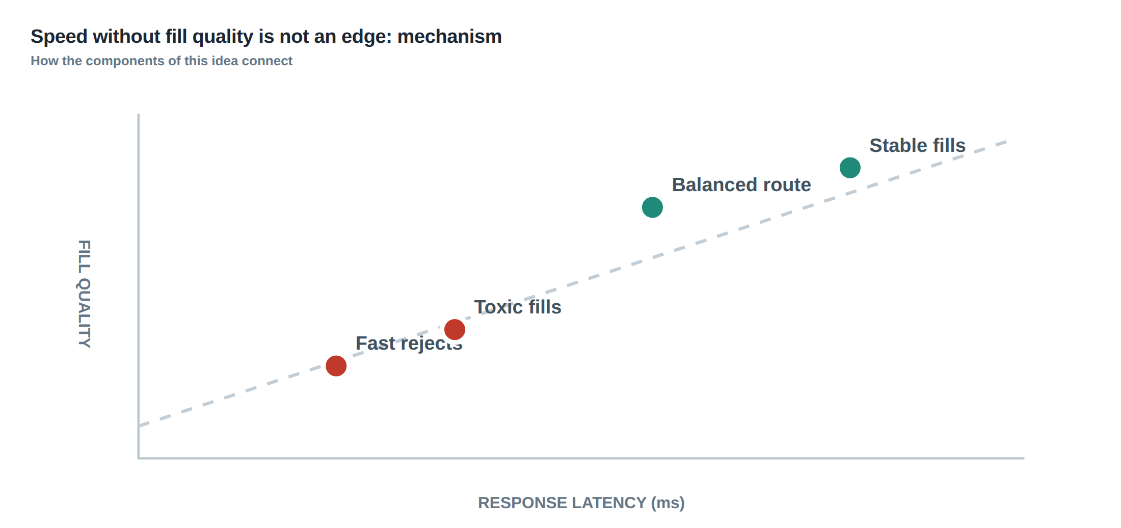
To evaluate whether latency truly adds value we must measure three intertwined metrics: the fill rate (the proportion of submitted orders that become executions), the realised spread (the price improvement or concession achieved on each fill), and the post‑fill price drift (how the market moves in the seconds after execution). These must be examined alongside the raw response time, otherwise a desk may chase a mirage of speed while the quality of the fills deteriorates. The core thesis, therefore, is that latency matters only when it improves executable prices, completion rates or risk outcomes.

A practical implication of this view is that an order’s lifetime cannot be judged by elapsed wall‑clock time alone. The system must continuously reassess whether the current queue position still justifies staying alive, given the expected spread capture, the probability of adverse selection, and the optionality of withdrawing before the market moves unfavourably. This dynamic assessment is what separates a genuinely profitable low‑latency strategy from a fragile one that collapses when market conditions change.

How the mechanism works, step by step

When a market participant sends a new limit order, the exchange places it at the back of the queue for the specified price level. The order’s “queue position” is a function of both price and arrival time; earlier orders have priority. As market participants submit marketable orders that cross the spread, the queue is depleted from the front. The order’s expected profit is the spread it will capture if it is executed before the queue is cleared, minus the expected adverse‑selection cost incurred if the price moves away while the order remains pending.

Step one is the latency‑induced time shift: a faster gateway reduces the interval between the trader’s decision and the order’s insertion into the queue. Step two is the queue‑value assessment: the system estimates, using recent order‑flow statistics, the probability that the order will be filled within a given horizon and the expected spread at that horizon. Step three is the risk‑adjusted decision: if the expected net spread (spread capture less adverse‑selection cost) exceeds a pre‑defined threshold, the order is kept alive; otherwise it is cancelled or amended.

Crucially, the queue‑value assessment must incorporate two additional signals. First, the rate of immediate rejections – often caused by risk checks, size limits or stale quotes – which inflate the apparent speed but do not contribute to execution. Second, the market‑state signal: volatility, order‑flow toxicity, and venue‑specific microstructure. In a high‑volatility regime the queue may be cleared within a few milliseconds, rendering a five‑millisecond latency improvement moot, while in a low‑volatility regime the same improvement may increase the chance of capturing a full tick of spread.

The system therefore operates as a feedback loop: latency improvements are only retained if, after the loop closes, the realised spread and fill probability have moved in the desired direction. If the loop shows a deterioration – for example, a rise in rejection rates or a higher incidence of adverse price movement after fills – the latency gain is deemed ineffective and the optimisation is rolled back.

A worked example with real numbers

Consider a statistical arbitrage strategy that posts passive limit orders on a highly liquid equity. The baseline latency from decision to exchange receipt is 20 ms. Over a ten‑minute window the strategy submits 10 000 orders, achieving a fill rate of 80 % (8 000 executions). The average realised spread per fill is 0.12 ticks, and the mean price drift in the first 500 ms after execution is a modest 0.20 ticks adverse to the trade. Rejection events – orders that are refused by the exchange before entering the queue – are rare, at 2 % of submissions.

After a hardware upgrade and a network optimisation the measured latency drops by five milliseconds to 15 ms. The raw response time improvement is confirmed by timestamp logs. However, the post‑upgrade statistics reveal a different picture: rejected orders double to 4 % (400 rejections), the fill rate falls to 70 % (6 300 executions), and the average realised spread shrinks to 0.07 ticks. Moreover, the adverse price movement after fills rises to 0.55 ticks, indicating that the strategy is now more often hitting the book when toxic flow is present. The net realised profit per order drops from 0.10 ticks (0.12 – 0.02) to 0.03 ticks (0.07 – 0.04), a three‑fold reduction despite the five‑millisecond speed gain.

The numbers illustrate that a pure latency metric is insufficient. The increase in rejections means the system is spending more cycles on orders that never reach the queue, while the lower fill rate and higher post‑fill drift show that the remaining executions are of poorer quality. In this scenario the five‑millisecond improvement is not progress; it is a net loss of edge because the faster decision does not translate into better executable prices or risk outcomes.

Where it breaks in live markets

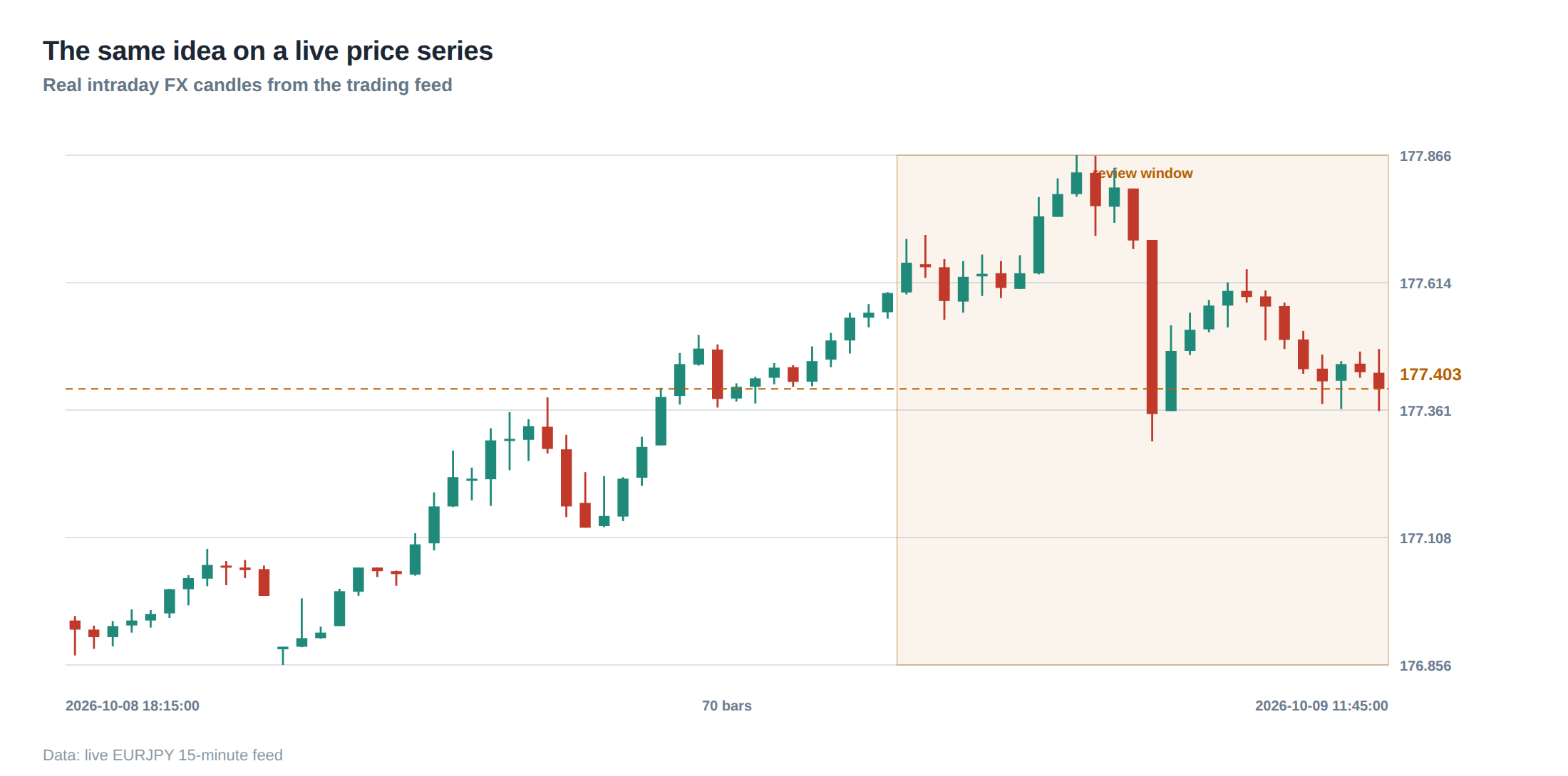
In live trading the relationship between speed and fill quality is fragile. Market microstructure can change within seconds: a sudden influx of informed orders, a news‑driven volatility spike, or a venue‑wide latency injection (for example, a temporary congestion event) can transform a benign queue into a toxic one. When the order flow becomes dominated by aggressive participants, the queue clears rapidly and the probability of a passive order being filled at a favourable price collapses. In such regimes a strategy that relies solely on being a few milliseconds faster may find its orders consistently rejected or executed at the worst possible price.

Another failure mode is the “venue‑specific latency trap”. Different exchanges and dark pools have heterogeneous matching engines, each with its own latency envelope and order‑type handling. An optimisation that reduces latency on one venue may inadvertently increase the proportion of orders routed to a venue where the order book is thin, leading to higher rejection rates and larger adverse selection. The same five‑millisecond gain can therefore manifest as a shift in execution venue rather than an improvement in execution quality.

Finally, the feedback delay between order submission and the market’s reaction can mask problems. Traders may observe a short‑term uplift in fill rate after a latency upgrade, but the true cost emerges later as the strategy’s exposure to adverse price moves accrues. Without a systematic post‑trade analysis that captures the realised spread and subsequent price drift, the desk may continue to allocate capital to a “fast” but ultimately unprofitable sub‑strategy.

The operating path, stage by stage

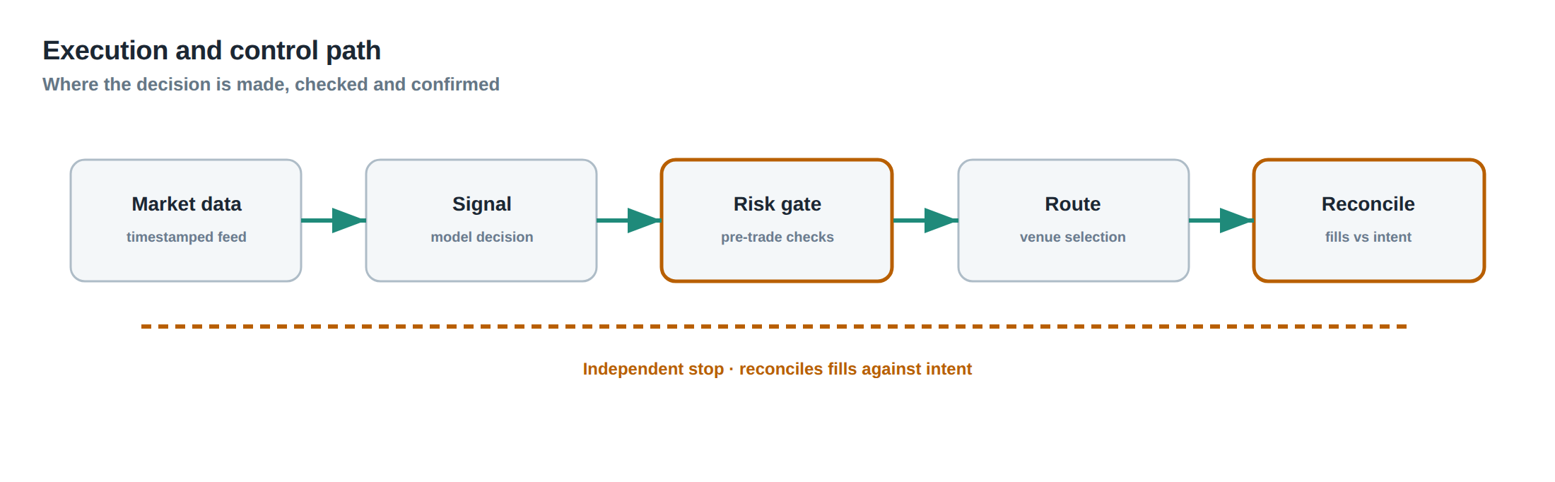
The operational workflow begins with a market‑state estimator that ingests real‑time metrics: order‑flow imbalance, realised volatility, and venue‑specific latency measurements. Based on this estimator, the order‑generation engine decides whether to submit a passive limit order, a marketable order, or to hold off entirely. Once the decision is made, the order is packaged and sent through the connectivity stack, where the latency optimisation layers (hardware acceleration, kernel bypass, co‑located routing) act.

Upon arrival at the exchange, the order enters the price‑time queue. The exchange’s risk engine may reject the order instantly; such rejections are logged and fed back to the risk‑adjustment module. If the order is accepted, it remains pending until either a marketable order consumes it, the order expires, or the system cancels it based on the dynamic queue‑value assessment. Each state transition – submission, acceptance, execution, cancellation, rejection – is timestamped to the microsecond.

The final stage is the post‑trade analytics block. Here the realised spread, fill rate, and post‑fill price drift are computed for each venue, session, and volatility regime. These metrics are compared against the pre‑trade expectations generated by the queue‑value model. If the realised metrics fall short, the system automatically flags the latency optimisation for review, potentially rolling back hardware changes or adjusting the order‑routing logic. This closed‑loop architecture ensures that speed improvements are retained only when they demonstrably enhance execution economics.

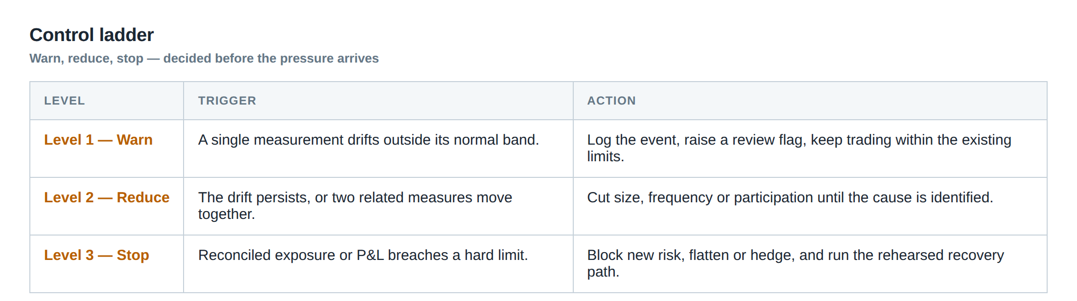
Controls that act before the damage

Preventative controls sit at two levels: the pre‑trade risk gate and the adaptive routing filter. The pre‑trade gate evaluates each candidate order against a set of thresholds derived from the queue‑value model – expected spread capture, maximum admissible adverse‑selection cost, and a ceiling on the probability of immediate rejection. If any metric falls outside its band, the order is either throttled, reduced in size, or converted to a marketable order.

The adaptive routing filter monitors venue‑specific latency and fill‑quality signals in real time. When a venue’s rejection rate spikes or its realised spread deteriorates beyond a dynamic tolerance, the filter automatically diverts traffic to alternative venues with more favourable queue conditions. Because the filter operates on sub‑second updates, it can prevent a flood of low‑quality fills that would otherwise accumulate during a transient market shock.

A third safeguard is the “latency‑impact audit”. Before any hardware or firmware change is deployed, a shadow‑run is executed where the new stack processes a copy of live market data while the production stack continues unchanged. The audit records fill‑rate, realised spread, and post‑fill drift for both streams, allowing a statistically robust comparison. Only if the new stack demonstrates a net improvement across these metrics is the change promoted to production.

How to measure whether it is working

Measurement must be multidimensional. First, compute the fill‑rate per venue and per session: filled orders divided by total submissions, excluding instantaneous rejections. Second, calculate the realised spread as the difference between the execution price and the prevailing mid‑price at the moment of fill, weighted by order size. Third, assess the post‑fill price drift by measuring the mid‑price movement over a fixed horizon (e.g., 500 ms) after each execution; the average of these drifts indicates the adverse‑selection exposure.

These three metrics should be plotted against latency histograms to visualise any correlation. A genuine edge appears when a reduction in median latency coincides with a higher realised spread and a lower adverse drift. Conversely, a flat or negative correlation signals that speed is not delivering economic benefit. The analysis must be stratified by volatility regime – low, medium, high – because the same latency improvement can have opposite effects in different market conditions. Finally, aggregate the per‑trade profit contribution (realised spread minus adverse drift) to obtain a net edge figure; this figure should be the primary KPI for any latency‑related project.

The portfolio view

From a portfolio perspective, each strategy contributes a marginal edge that is a function of its execution quality. When latency upgrades are rolled out, the portfolio manager should monitor the change in aggregate realised spread across all strategies, not just the headline latency reduction. If the net contribution to portfolio Sharpe ratio declines, the upgrade is likely harming the overall edge despite its technical success.

Risk budgeting also benefits from the queue‑value lens. Strategies that rely heavily on passive liquidity provision allocate a larger portion of their risk budget to adverse‑selection exposure. By quantifying how latency affects that exposure, the manager can re‑balance capital towards strategies whose execution quality improves with speed, and away from those that become more toxic. Over longer horizons, the cumulative effect of small latency‑induced fill‑quality degradations can erode capital, especially in high‑turnover portfolios where execution cost is a significant component of total return. Therefore, the portfolio view reinforces the core thesis: speed without fill quality is not an edge, and every latency decision must be justified by its impact on realised spread, fill probability, and risk outcomes.

In practice, a disciplined desk will treat latency as a lever rather than a goal, pulling it only when the downstream metrics confirm a positive contribution to the portfolio’s risk‑adjusted return.

What aspect of your own execution workflow would benefit most from a systematic, queue‑value‑based latency assessment?

About the research behind this lesson

The seminar frames electronic markets as price-time-priority queues. It separates queue value into spread capture versus adverse-selection cost and the option value of retaining a place in line.

Applied to this lesson: An order lifetime therefore cannot be based on elapsed time alone: the system must reassess whether its queue position, expected spread and adverse-selection risk still justify keeping the order alive.

Explore PULSE: System details

PULSE live account: Verify the live account on FX Blue

Live chat and updates: Telegram @xtrskhft

Source: High-Frequency Trading and Modern Market Microstructure

Educational content only. Trading leveraged products involves risk.