October 5, 2026

What this problem really is

Statistical‑arbitrage strategies are built on the belief that two or more instruments that have moved together in the past will continue to do so long enough for a trader to capture a mean‑reverting spread. The core assumption is that the historical co‑movement is a reliable proxy for future dynamics. In practice this assumption is fragile because the statistical relationship is observed on a finite sample, under a particular market regime, and without the influence of the trader’s own capital. When a sizeable position is taken, the act of trading can alter the very dynamics that justified the trade, turning a seemingly stationary spread into a drifting one. Consequently, the risk is not merely that the spread fails to converge, but that the model itself is misspecified – a model‑risk trade. The danger is amplified when the model ignores regime shifts, common‑factor exposures, and the full cost structure of the trade.

The problem is therefore two‑fold. First, the statistical test that declares a spread “stationary” is usually based on a single regime, ignoring that markets cycle through high‑volatility, low‑volatility, and structural‑change periods. Second, even if the spread is truly stationary, the trader’s capital can push the price away from its equilibrium, especially when the strategy relies on leverage, borrowing, or short‑selling. The result is a feedback loop where the model’s predictions become self‑defeating.

A proper assessment of statistical arbitrage must therefore treat the spread as a stochastic process embedded in a broader market environment, and must explicitly model the cost of capital, the half‑life of reversion, and the possibility that the underlying co‑integration vector may rotate. Only then can a trader decide whether the expected profit compensates for the model‑risk exposure.

How the mechanism works, step by step

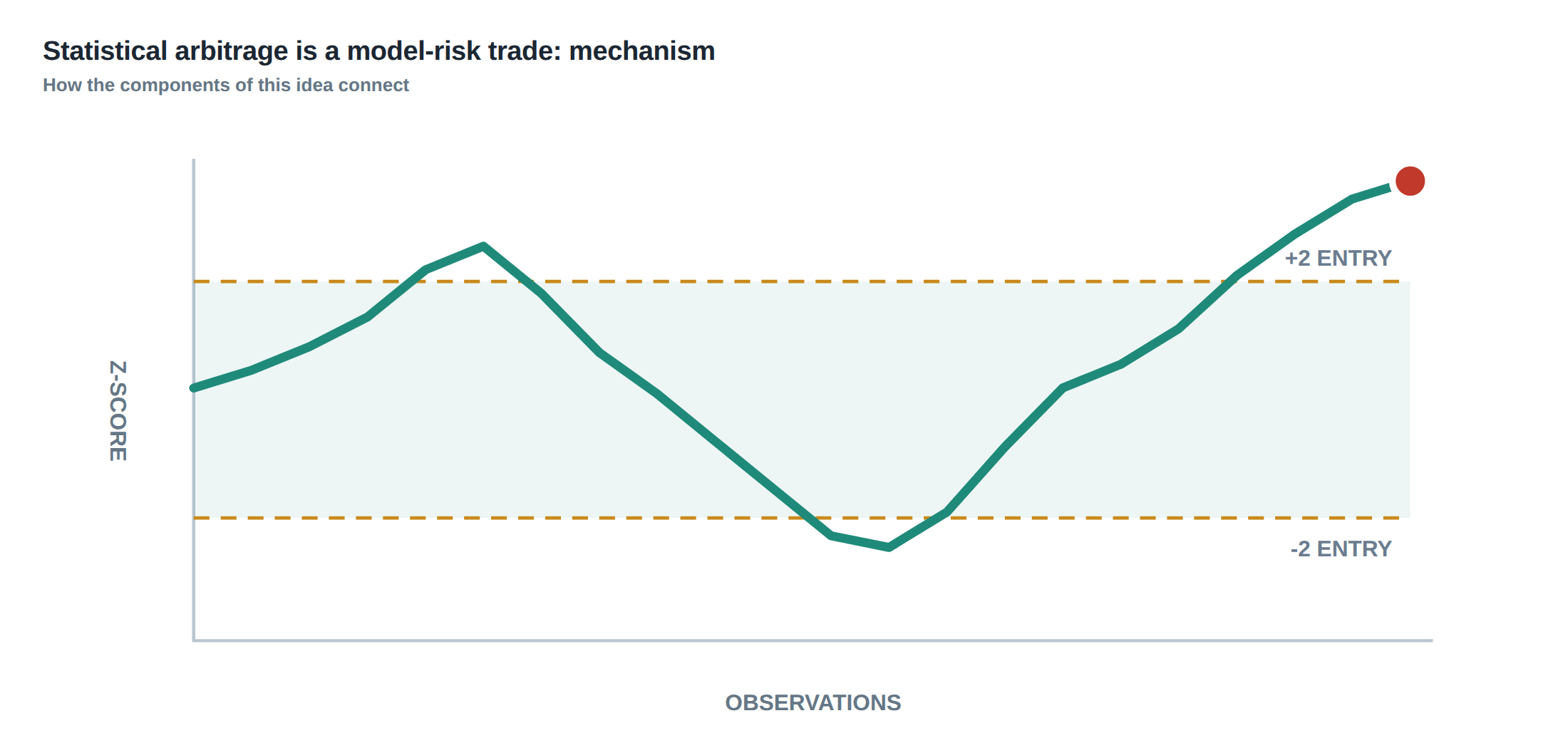
The first step is to identify a pair or a basket of securities that appear to move together. A standard approach is to run a Johansen test or an Engle‑Granger regression on a rolling window of, say, 250 trading days, and to extract the residual series – the spread. The residual is then examined for stationarity using an Augmented Dickey‑Fuller test, and the half‑life of mean reversion is estimated from the autoregressive coefficient.

Next, the spread is decomposed into two components. The common‑factor exposure captures the part of the price movement that can be explained by market‑wide drivers such as the S&P 500 index, sector ETFs, or macro‑economic variables. The residual spread behaviour is what remains after regressing the raw spread against these factors. By isolating the residual, the trader removes the risk that a broad market move will be misinterpreted as a convergence signal.

The third step introduces the cost layer. Borrowing costs for short positions, funding rates for leveraged long exposure, turnover‑related transaction costs, and execution slippage are all quantified. These are subtracted from the theoretical mean‑reversion profit to obtain a net expected return.

Finally, the trader sets two complementary exit criteria. A price stop is triggered when the spread’s z‑score reaches a pre‑defined threshold on the opposite side of the mean, indicating that the convergence expectation has been exhausted or reversed. A time stop is activated if the spread has not moved a statistically significant amount within a multiple of its half‑life, signalling that the underlying relationship may have weakened. Both stops are enforced simultaneously, ensuring that the position is closed either by price or by elapsed time.

A worked example with real numbers

Consider a pair trade between two large‑cap technology stocks, AlphaTech (AT) and BetaSoft (BS). Over the past 300 days the log‑price ratio \(R_t = \ln(P^{AT}_t) – \ln(P^{BS}_t)\) has a sample mean of 0.012 and a standard deviation of 0.025. An ADF test on the residuals of the regression against the market index returns a p‑value of 0.01, indicating stationarity at the 1 % level. The estimated AR(1) coefficient is 0.85, giving a half‑life of \(\frac{\ln(2)}{-\ln(0.85)} \approx 4.2\) days.

The trader computes the z‑score of the current spread as \(\frac{R_t – \mu}{\sigma} = \frac{0.045 – 0.012}{0.025} = 1.32\). The model’s entry rule is a z‑score beyond +1.5, so the signal is not yet triggered. However, on day 180 a sudden earnings surprise pushes AT up, widening the spread to a z‑score of 2.1. The model therefore initiates a short position in AT and a long position in BS, each sized to a dollar exposure of \$5 million.

The borrow cost for shorting AT is 2.5 % annualised, which on a 5‑day holding period translates to a cost of \(\$5\,\text{m} \times 0.025 \times \frac{5}{252} \approx \$2\,500\). Funding the long leg in BS at the repo rate of 1.8 % adds another \(\$5\,\text{m} \times 0.018 \times \frac{5}{252} \approx \$1\,800\). Expected turnover is 0.3 % per side, giving a combined execution cost of \(\$5\,\text{m} \times 0.003 \times 2 = \$30\,000\).

The theoretical profit from mean reversion, assuming the spread returns to its mean within one half‑life, is \(\Delta R = 2.1 – 0 = 2.1\) standard deviations, i.e. a price move of \(2.1 \times 0.025 = 0.0525\) in log‑terms. Converting to price, this corresponds to a profit of roughly \(\$5\,\text{m} \times 0.0525 \approx \$262\,500\) on each leg, or \$525 000 total. Subtracting borrowing, funding and execution costs leaves a net expected profit of about \$491 000.

Because the entry z‑score is well above the usual threshold, the trader applies a widening of the position size to reflect the higher uncertainty. Instead of the full \$5 million per leg, only 70 % of the nominal exposure is taken, reducing the net expected profit to roughly \$344 000 while also limiting the downside if the spread fails to converge.

A price stop is set at a z‑score of –0.5, which would close the trade if the spread overshoots the mean in the opposite direction. A time stop is programmed at 3 × half‑life, i.e. 12.6 days. If after 13 days the spread has not moved more than 0.5 σ towards the mean, the position is liquidated regardless of price.

In this example the wide z‑score could have been a genuine arbitrage opportunity, a sign of a structural break, or simply a data glitch. By scaling the exposure down and by imposing both price and time stops, the trader embeds a hedge against each of those possibilities.

Where it breaks in live markets

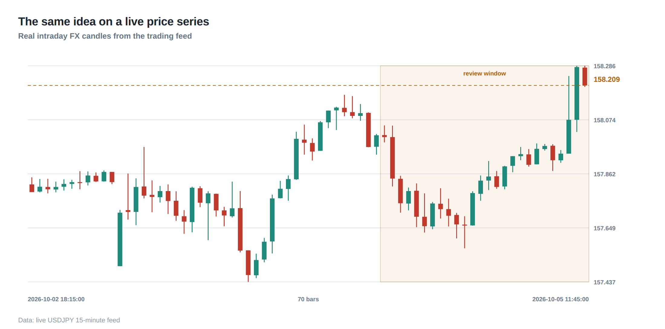
The theoretical framework assumes that the spread follows a linear Ornstein‑Uhlenbeck process with constant parameters. Real markets, however, display abrupt regime shifts caused by macro‑economic announcements, changes in market microstructure, or the entry of large institutional participants. When a regime change occurs, the estimated half‑life can double or halve within a few days, rendering the previously calibrated stop levels either too tight or too lax.

Liquidity dries up during stress periods, causing execution costs to spike well beyond the 0.3 % turnover assumption. The order‑book depth may collapse, and the price‑time‑priority queue that underpins the spread capture becomes dominated by adverse‑selection risk. In such environments the expected spread may be captured only after a significant delay, eroding the option value of staying in line.

Borrow and funding rates are not static; they widen sharply when the market perceives a particular stock as a “hard‑to‑borrow” short. If the short leg of the pair becomes scarce, the cost of maintaining the position can exceed the anticipated convergence profit before the spread even begins to revert.

Finally, data quality issues – stale quotes, corporate actions not yet reflected, or erroneous timestamps – can produce spurious outliers that masquerade as extreme z‑scores. If the model does not include a sanity‑check filter, a trader may allocate capital to a non‑existent arbitrage, exposing the portfolio to unnecessary loss.

The operating path, stage by stage

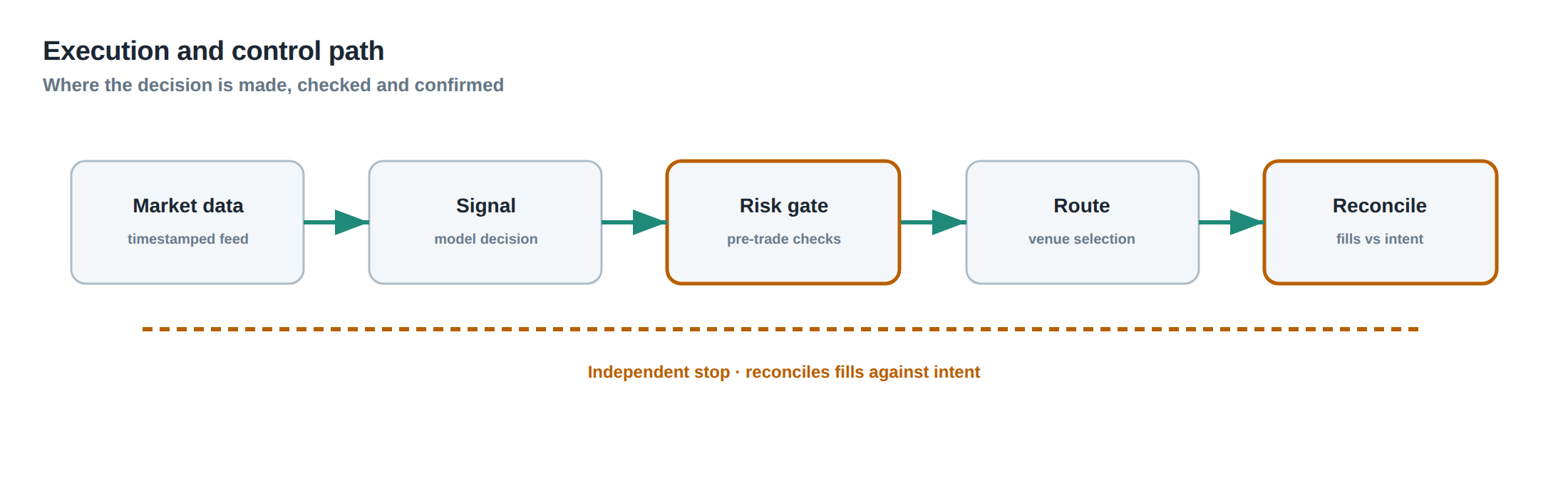
The first stage is data ingestion and cleansing. Prices are aligned to a common timestamp, corporate actions are adjusted for, and missing bars are interpolated only when the gap is less than five minutes; otherwise the observation is discarded. The second stage is factor extraction, where the market and sector indices are regressed against each instrument to obtain factor loadings. The residual spread is then computed by subtracting the factor‑based component from the raw price ratio.

Stage three involves statistical testing. The ADF statistic and its critical values are calculated on a rolling window, and the half‑life is derived from the AR(1) coefficient. If the p‑value exceeds 0.05 or the half‑life exceeds a pre‑set maximum of 15 days, the pair is flagged as non‑stationary and removed from the candidate pool.

Stage four is risk budgeting. The model aggregates borrow, funding, turnover and slippage estimates into a single cost per dollar of exposure. It then compares the net expected return to a risk‑adjusted hurdle rate, typically set at 8 % annualised. Only pairs that clear this hurdle are passed to the execution engine.

Stage five is order placement. The algorithm submits limit orders at the best bid or ask, depending on the direction of the trade, and monitors the queue position in real time. If the queue depth falls below a threshold, the order is cancelled and re‑submitted at a more aggressive price. The system continuously re‑evaluates the expected spread, the adverse‑selection probability and the remaining time‑to‑stop, deciding whether to keep the order alive.

The final stage is post‑trade analytics. realised P&L, slippage, and the deviation of the actual half‑life from the forecast are recorded. These metrics feed back into the model‑validation loop, updating the regime‑detection filters and the exposure caps for future trades.

Controls that act before the damage

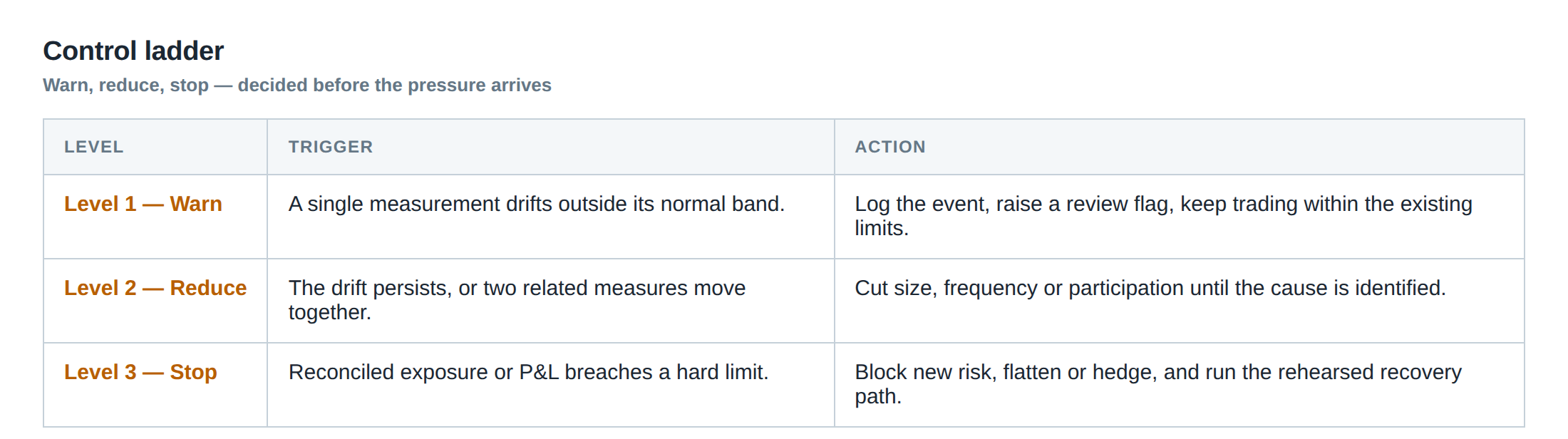
A layered control framework is essential to prevent model‑risk from materialising. The first line of defence is a regime‑detection filter that monitors volatility, correlation, and the eigenvalue spectrum of the factor covariance matrix. When a shift is detected, the half‑life estimate is recomputed on a shorter window and the exposure cap for the affected pair is automatically reduced to 30 % of its usual level.

The second line is a real‑time cost monitor. It tracks the borrow rate, the repo rate and the realised execution cost per trade. If any of these metrics exceed a pre‑defined multiplier of their historical average – for example, a 150 % increase in borrow cost – the system aborts the entry and flags the pair for review.

The third line is a position‑size governor that incorporates the width of the z‑score. A wide z‑score (greater than 2.5) triggers a scaling factor that reduces the nominal exposure in proportion to the distance from the mean, thereby limiting the capital at risk when the signal may be contaminated by structural change or bad data.

The fourth line is the dual stop mechanism. The price stop is set at a modest opposite‑side z‑score of –0.5, while the time stop is set at three half‑lives. If either condition is met, the trade is liquidated immediately, preventing the accumulation of adverse‑selection losses that would otherwise erode the option value of staying in the queue.

Together these controls create a pre‑emptive shield that forces the system to reassess the validity of the spread before capital is fully committed, and to unwind the position as soon as the underlying assumptions become questionable.

How to measure whether it is working

Performance measurement must separate pure statistical‑arbitrage returns from the cost and risk components. The primary metric is the Sharpe ratio of the residual spread after deducting borrow, funding and execution costs. A secondary metric is the realised half‑life compared with the forecast half‑life; a systematic bias indicates that the stationarity assumption is deteriorating.

Turnover adjusted return on capital (Roc) is calculated by dividing net profit by the average gross exposure, providing a view of how efficiently capital is being deployed. The hit‑ratio – the proportion of trades that close within one half‑life and achieve a profit greater than the total cost – offers a direct gauge of the model’s predictive power.

Risk metrics include the maximum drawdown of the pair‑level equity curve and the exposure‑adjusted VaR, which incorporates the borrowing cost volatility. Monitoring the frequency of time‑stop activations versus price‑stop activations helps to identify whether the regime‑detection filter is too aggressive or too lax.

Finally, a regression of realised P&L against the forecasted mean‑reversion profit can be performed periodically. The slope should be close to one and the intercept near zero; deviations signal that either the cost model or the statistical model has drifted.

The portfolio view

When multiple pairs are combined, the portfolio’s exposure to common factors must be managed explicitly. By aggregating the factor loadings of each pair, the desk can enforce a net‑zero market beta, ensuring that the portfolio’s performance is driven primarily by residual spread capture rather than by broad market moves.

Diversification across sectors, liquidity tiers and regime‑sensitivity profiles reduces the probability that a single structural break wipes out a large portion of the capital. The portfolio’s aggregate half‑life distribution should be monitored; a concentration of very short half‑lives may indicate over‑trading, while a preponderance of long half‑lives could signal that the desk is chasing marginal opportunities with higher model‑risk.

Capital allocation is performed on a risk‑budget basis. Each pair is assigned a volatility‑scaled budget that respects the overall VaR limit of the desk. When a pair’s exposure cap is reduced because of a regime shift, the freed capital is re‑allocated to pairs that remain in a favourable regime, preserving the overall utilisation rate.

The ultimate test of the portfolio is its ability to generate a stable, positive alpha after all costs, while keeping the model‑risk contribution to the total risk budget below a pre‑agreed threshold – typically 20 % of the overall VaR. Continuous back‑testing, live‑monitoring of regime indicators and strict adherence to the dual stop framework are the pillars that keep the portfolio from being eroded by the very statistical relationships it seeks to exploit.

Do you have a systematic process for detecting when a historically stationary spread has entered a new regime, and how would you adjust your exposure in real time?

About the research behind this lesson

The seminar frames electronic markets as price-time-priority queues. It separates queue value into spread capture versus adverse-selection cost and the option value of retaining a place in line.

Applied to this lesson: An order lifetime therefore cannot be based on elapsed time alone: the system must reassess whether its queue position, expected spread and adverse-selection risk still justify keeping the order alive.

Explore PULSE: System details

PULSE live account: Verify the live account on FX Blue

Live chat and updates: Telegram @xtrskhft

Source: High-Frequency Trading and Modern Market Microstructure

Educational content only. Trading leveraged products involves risk.