October 13, 2026

What this problem really is

Statistical‑arbitrage strategies are built on the assumption that two or more instruments have a long‑run co‑movement that can be expressed as a spread. The spread is observed to revert to a mean in historical data, and the trader bets that the same reversion will occur after capital is deployed. In practice the relationship is fragile: the statistical properties that justified the trade may disappear the moment a sizeable order is placed, when market participants adjust their behaviour, or when the underlying economic regime shifts. The risk is not a simple “model error” but a model‑risk trade – the model tells you a spread is stationary, yet the act of trading can invalidate that stationarity.

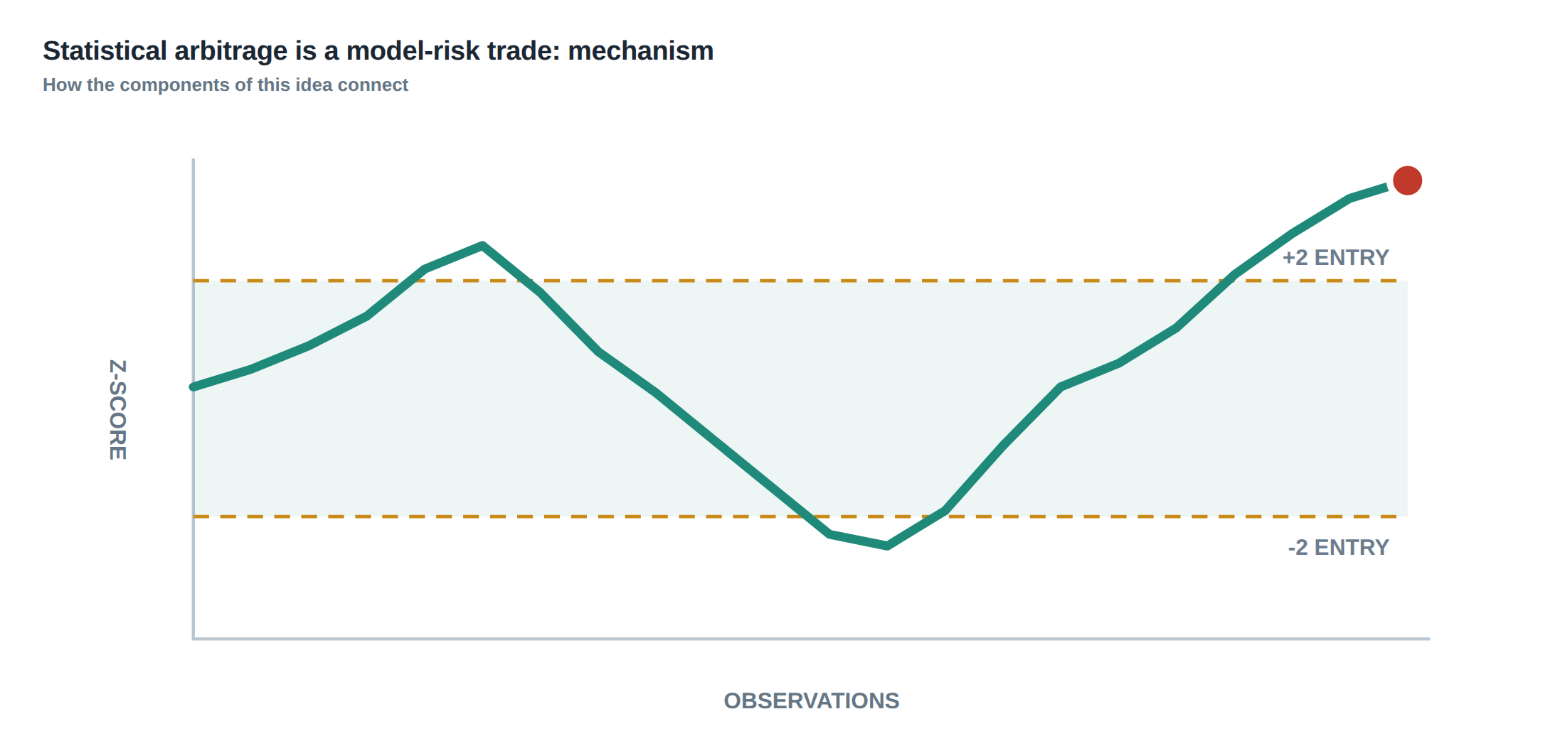
When the spread widens beyond a conventional z‑score threshold, the trader interprets the move as an “opportunity”. That same widening can also be a warning sign of structural change, data corruption, or a breakdown in the assumed common factor. The key is to recognise that the historical co‑movement does not guarantee convergence after the position is taken, because the market’s microstructure, funding conditions and the trader’s own impact all feed back into the spread dynamics.

Consequently, a robust statistical‑arbitrage framework must treat the spread as a stochastic process whose parameters are themselves stochastic. The model must be continuously re‑estimated, and the trade must be equipped with hard limits that can be triggered by either price movement or the passage of time, rather than relying solely on the original statistical signal.

How the mechanism works, step by step

The first step is to identify a pair or basket of securities whose price histories exhibit a high degree of correlation after removing a common factor, usually a market index or sector return. A regression or a principal‑component analysis isolates the common factor, leaving a residual series that is interpreted as the spread. The residual is then tested for stationarity using Augmented Dickey‑Fuller or Phillips‑Perron tests across several historical regimes – for example, pre‑2008, post‑2008, and the most recent two‑year window. If the test rejects the unit‑root hypothesis in each regime, the spread is deemed stationary, and the half‑life of mean reversion is estimated from the autoregressive coefficient.

Next, the trader builds a trading rule that converts the spread into a z‑score by subtracting the long‑run mean and dividing by the rolling standard deviation. A long position is opened when the z‑score falls below a negative threshold (e.g., –2) and a short when it rises above a positive threshold (e.g., +2). The size of each leg is calibrated to the volatility of the spread, the capital allocated to the strategy, and the cost of borrowing the short leg. Funding costs, turnover, and execution slippage are added to the expected profit‑and‑loss (P&L) to obtain a net edge.

Finally, the order is submitted to an electronic limit‑order book that operates on a price‑time priority queue. The queue position carries an option‑like value: staying in line may capture the spread if the price moves favourably, but it also exposes the trader to adverse selection – the risk that a better‑informed participant removes liquidity and forces an unfavourable fill. Because the queue value erodes over time, the system must continuously reassess whether the expected spread capture still outweighs the adverse‑selection cost, and decide whether to cancel or amend the order.

A worked example with real numbers

Consider a pair of large‑cap equities, AlphaCorp (ALP) and BetaLtd (BET), whose daily closing prices over the past three years have a correlation of 0.92 after adjusting for the market index. A simple OLS regression of ALP on BET yields a hedge ratio of 1.18, and the residual series – the spread – shows an Augmented Dickey‑Fuller statistic of –4.3 in the full sample, comfortably below the 5 % critical value. The estimated autoregressive coefficient is 0.85, implying a half‑life of ln(2)/|ln(0.85)| ≈ 4.3 days.

On a particular Monday the rolling mean of the spread is 0.015 and the rolling standard deviation is 0.006. The observed spread is –0.018, giving a z‑score of (–0.018 – 0.015)/0.006 ≈ –5.5. The model flags a strong short‑side opportunity: the spread is far below its mean and, given the half‑life, should revert within a week. The trader decides to allocate £2 million of capital, scaling the position by the spread’s volatility: the notional of ALP to buy is (£2 m × 0.6) ≈ £1.2 m, and the short notional of BET is (£2 m × 0.4) ≈ £0.8 m, reflecting the hedge ratio and the relative liquidity of each stock.

Borrowing BET for the short leg costs 0.35 % per annum, funding ALP costs 0.10 % per annum, and the expected turnover is three round‑trips per month, each incurring an execution cost of 2 bps. Adding these, the annualised cost of the position is roughly 12 bps. The projected gross mean‑reversion profit, based on the half‑life, is 45 bps, leaving a net edge of 33 bps. However, the z‑score of –5.5 also raises a flag: such an extreme deviation could stem from a data glitch, a sudden macro‑event, or a breakdown in the hedge ratio. The trader therefore caps the exposure at 50 % of the target notional and sets a price stop at a z‑score of –7 and a time stop of three days. If either limit is breached, the order is cancelled, regardless of the original signal.

Where it breaks in live markets

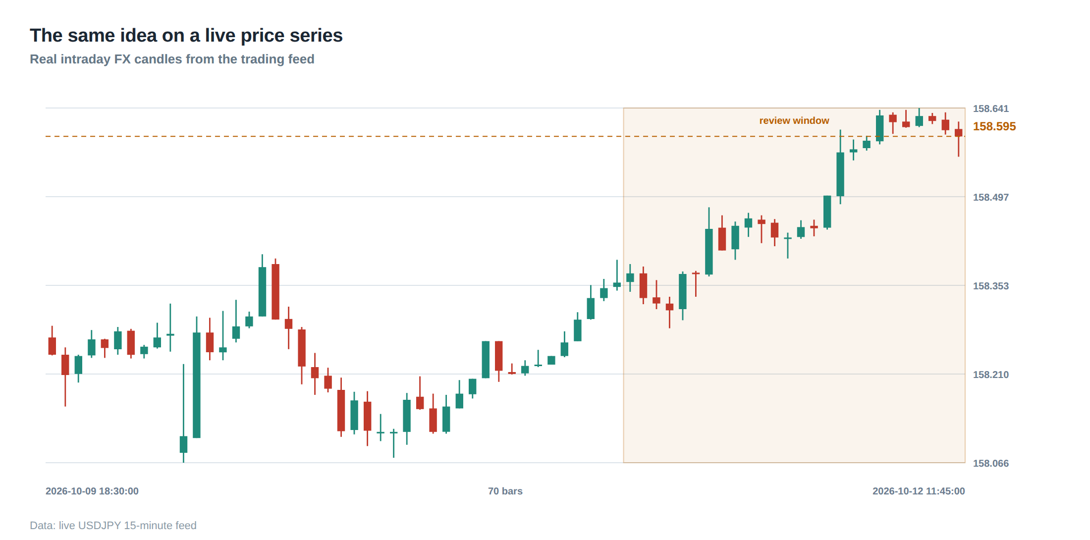
The moment a sizeable order reaches the limit‑order book, the market’s microstructure reacts. Other participants observe the added depth on one side of the spread and may adjust their own quoting strategies, either by widening the quoted spread or by stepping ahead in the queue. This “queue‑jumping” behaviour erodes the expected capture of the spread because the trader’s order is displaced further down the line, increasing the expected waiting time before execution.

Funding conditions can shift abruptly. If the short leg is a hard‑to‑borrow security, the borrow rate may spike from 0.35 % to 2 % within a few hours, instantly turning a previously profitable trade into a loss‑making one. Similarly, a sudden increase in turnover – perhaps triggered by a news release that moves both securities – raises execution costs beyond the model’s static estimate, compressing the net edge.

Regime changes are the most insidious. The stationarity test that held over the past three years may fail after a structural shift such as a merger, a change in market‑making rules, or a macro‑policy shock. The half‑life, which was 4.3 days under normal conditions, can lengthen dramatically, meaning the spread may not revert within the planned horizon. If the trader’s system does not detect the change, the position may be held until the time stop expires, incurring funding costs without the expected mean‑reversion profit.

The operating path, stage by stage

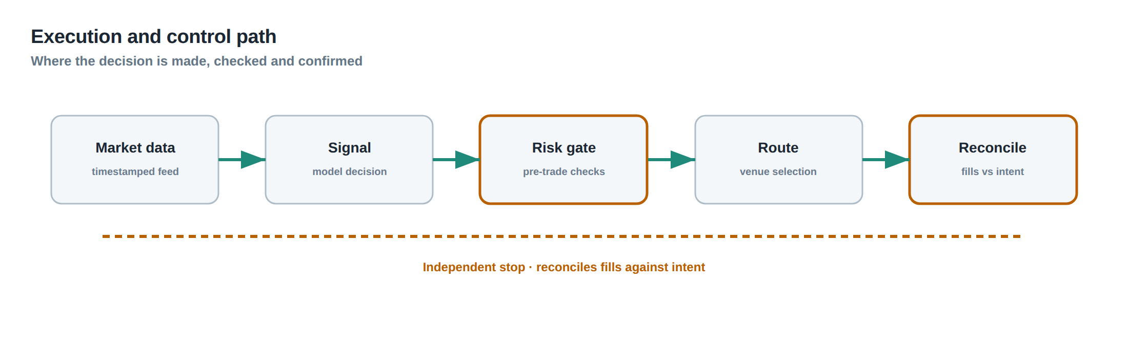
Stage one is data ingestion and factor extraction. Prices are cleaned, corporate actions are adjusted, and the common market factor is removed to produce the residual spread. Stage two is statistical validation, where unit‑root tests, rolling half‑life calculations and regime‑segmented analyses confirm that the spread behaves like a mean‑reverting process. Stage three translates the statistical signal into an actionable order: the spread is normalised, thresholds are applied, and the size of each leg is computed after accounting for borrowing costs and turnover expectations.

Stage four is order placement. The limit order is routed to the exchange with a price that reflects the current spread and a time‑in‑force that respects the pre‑defined time stop. The order sits in the price‑time priority queue, and the system continuously monitors the queue depth, the expected adverse‑selection cost, and the residual spread’s deviation. Stage five is risk enforcement: if the spread moves beyond the price stop, if the time stop elapses, or if the exposure exceeds the cap set for a regime change, the order is cancelled or scaled down. Stage six is post‑trade analysis, where realised P&L, execution slippage and funding charges are recorded and fed back into the statistical models for the next calibration cycle.

Each stage contains feedback loops. For example, a widening of the spread that pushes the z‑score toward the price stop also triggers a re‑estimation of the half‑life; a sudden increase in borrow cost forces a recalculation of the net edge, which may lead to an immediate exposure reduction before the price stop is reached. The architecture therefore resembles a control system with both feed‑forward and feedback components, designed to keep the trade within a safe operating envelope.

Controls that act before the damage

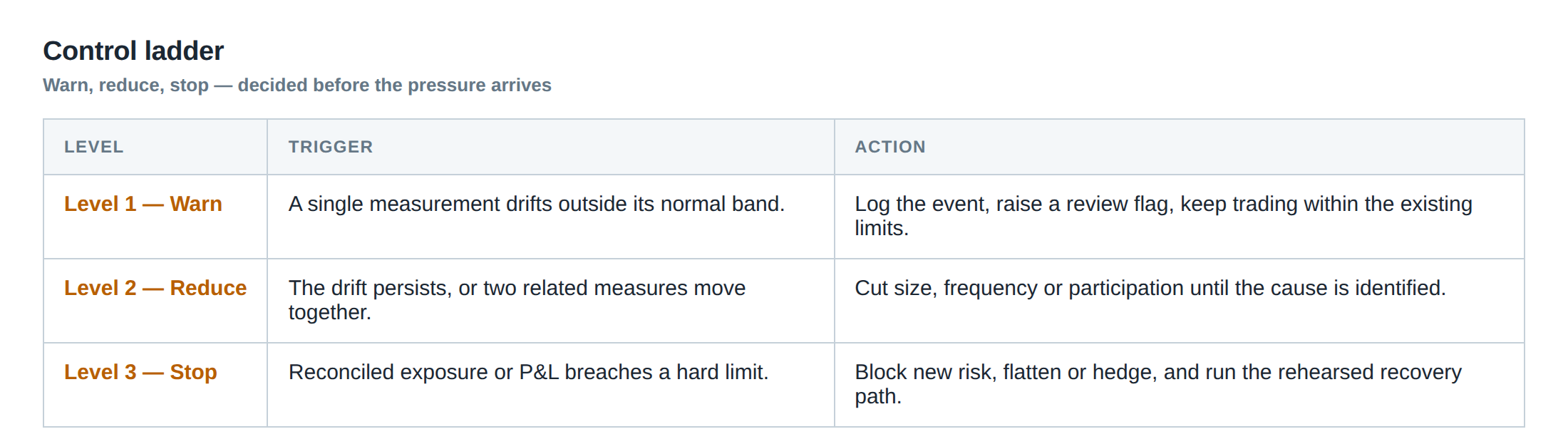
The first line of defence is a pre‑trade exposure cap that is linked to the statistical confidence of the spread. When the rolling p‑value of the stationarity test exceeds 0.10, the system automatically reduces the notional to a fraction of the baseline, recognising that the evidence for mean reversion is weakening. A second control is the dynamic borrowing‑cost filter: the system pulls real‑time borrow rates from the securities lending market and rejects any trade where the implied funding charge exceeds a preset proportion of the expected gross profit.

A third safeguard is the queue‑value monitor. By estimating the expected time to fill based on current queue depth and order‑flow intensity, the system assigns an option‑like value to the order’s position in line. If the estimated value falls below a threshold – for instance, when the expected adverse‑selection loss exceeds 70 % of the projected spread capture – the order is withdrawn before it incurs further cost.

Finally, the dual stop mechanism – a price stop based on the z‑score and a time stop based on the half‑life – ensures that a trade does not linger in an unfavourable state. The time stop is often set at 1.5 × the estimated half‑life; if the spread has not moved appreciably by that point, the probability of reversion within a reasonable horizon is low, and the position is closed to preserve capital.

How to measure whether it is working

Performance measurement begins with the realised Sharpe ratio of the spread‑return series after costs. However, a more granular view separates the components: the gross mean‑reversion return, the funding charge, the execution slippage, and the adverse‑selection loss derived from queue displacement. By tracking each component over time, the desk can detect whether the statistical model is still delivering the expected edge or whether any cost element has drifted upward.

Another key metric is the hit‑rate of the dual stops. A high proportion of trades that hit the price stop may indicate that the z‑score threshold is too aggressive, or that the spread has entered a new regime. Conversely, frequent time‑stop exits suggest that the half‑life estimate is overly optimistic. The average duration of a trade, measured against the theoretical half‑life, provides a sanity check on the model’s timing assumptions.

Finally, the stability of the hedge ratio is monitored through a rolling regression. Large swings in the coefficient – for example, a change from 1.18 to 0.95 over a month – signal that the common‑factor exposure is drifting, and that the residual spread may no longer be pure. When such drift is detected, the system either re‑optimises the hedge or temporarily suspends trading on that pair until the relationship stabilises.

The portfolio view

From a portfolio perspective, each statistical‑arbitrage leg is treated as a micro‑strategy that contributes to an overall market‑neutral exposure. The aggregate of all pairs should have a net beta close to zero, limiting directional risk. Nevertheless, the portfolio retains a residual exposure to common‑factor shocks that are not fully captured by the regression, as well as to liquidity shocks that affect multiple securities simultaneously.

Risk budgeting allocates a maximum capital drawdown to the statistical‑arbitrage block, often expressed as a percentage of the total equity. Within that block, each pair receives a risk‑adjusted allocation based on its historical Sharpe and its current confidence level – the latter derived from the latest stationarity p‑value and borrow‑cost spread. Correlation among spreads is also monitored; if several pairs become highly correlated, the effective diversification drops, and the portfolio manager may prune the most redundant legs.

The final layer of oversight is the stress‑test framework. Scenarios that spike borrow rates, widen spreads, or increase queue depth are simulated to see how the combined exposure would behave. The results feed back into the exposure caps and stop‑loss parameters, ensuring that the portfolio can survive extreme but plausible market conditions without breaching the pre‑agreed risk limits.

Do you have a systematic process in place to reassess queue position, funding costs and spread stationarity before a trade is allowed to run its full course?

About the research behind this lesson

The seminar frames electronic markets as price-time-priority queues. It separates queue value into spread capture versus adverse-selection cost and the option value of retaining a place in line.

Applied to this lesson: An order lifetime therefore cannot be based on elapsed time alone: the system must reassess whether its queue position, expected spread and adverse-selection risk still justify keeping the order alive.

Explore PULSE: System details

PULSE live account: Verify the live account on FX Blue

Live chat and updates: Telegram @xtrskhft

Source: High-Frequency Trading and Modern Market Microstructure

Educational content only. Trading leveraged products involves risk.