October 6, 2026

What this problem really is

A “lot” in most electronic desks is a fixed notional – one contract, one thousand shares, one standardised futures unit. The intuitive belief is that buying one lot always carries the same amount of risk, because the size of the position never changes. In practice the risk attached to that lot is a function of the instrument’s price‑movement volatility. When volatility expands, the same notional can swing many times the profit‑and‑loss (P&L) that would be expected in a calm market. The consequence is a risk budget that is no longer stable: a strategy calibrated on a low‑volatility regime will suddenly breach its VaR or expected shortfall limits when the market becomes more turbulent. The problem is therefore not a flaw in the lot definition but a mismatch between a static quantity and a dynamic risk environment.

The issue is amplified for high‑frequency or intra‑day strategies where the holding period is measured in seconds. A single tick move that is negligible on a daily horizon can represent a sizeable fraction of the daily standard deviation when the market is jittery. Consequently, the “one lot = one unit of risk” assumption collapses, and the desk must treat the lot as a variable exposure that is re‑scaled each time the volatility estimate changes.

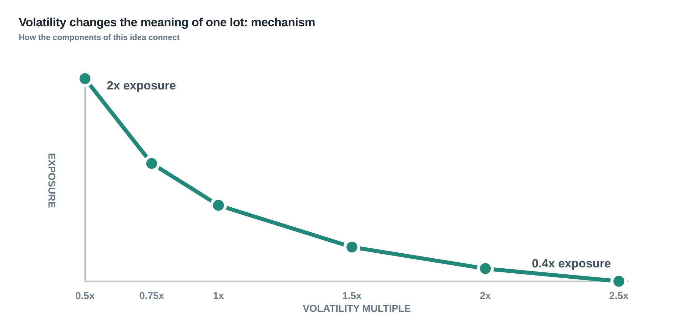
The core thesis is that a fixed quantity produces unstable risk when the instrument’s typical movement changes. The solution is to let the size of the position be a function of a forward‑looking volatility forecast, thereby normalising the risk contribution of each lot across regimes.

How the mechanism works, step by step

The first step is to obtain a volatility estimate that reflects the price dynamics over a horizon relevant to the strategy. For a 5‑minute scalping algorithm the estimate might be the realised standard deviation of 5‑minute returns over the previous 60 minutes. The second step is to decide how much capital the strategy is allowed to risk per trade – the risk budget – expressed as a fraction of the total equity, for example 0.5 % per execution.

With those two numbers the exposure is calculated by the inverse‑volatility rule:

\[ \text{Target Notional}= \frac{\text{Risk Budget}}{\sigma_{\text{est}}}\times K \]

where \(\sigma_{\text{est}}\) is the volatility estimate and \(K\) is a scaling constant that converts a standard‑deviation unit into a monetary loss (for instance, the price of one point multiplied by the contract multiplier). The rule ensures that, regardless of the current volatility, the expected one‑sigma loss of the trade equals the pre‑specified budget.

A look‑back window must be chosen to balance responsiveness and turnover. A very short window reacts quickly to spikes but produces noisy estimates, leading to excessive re‑sizing and higher transaction costs. A very long window smooths the estimate but lags behind abrupt regime shifts, exposing the desk to sudden over‑allocation. The optimal window is typically found by back‑testing the trade‑off between realised risk and turnover, often landing in the range of 30‑120 observations for intra‑day horizons.

The third step is to enforce floors and caps on the calculated notional. A floor prevents the algorithm from shrinking to a size that is uneconomical given fixed costs, while a cap stops the position from growing to a level that would breach market impact limits or regulatory position caps. The floor and cap are expressed in lots, for example a minimum of 1 contract and a maximum of 20 contracts.

Finally, the algorithm must recognise periods when volatility estimates become unreliable – for example during market halts, news spikes, or illiquid trading windows. In those circumstances a discretionary reduction factor, often a multiplicative 0.5 or 0.25, is applied to the target notional regardless of the raw estimate. This safety‑layer prevents the system from taking a full‑size position when the statistical foundation of the estimate is compromised.

A worked example with real numbers

Assume a futures contract with a point value of US$10 and a contract multiplier of 1. The desk has allocated a risk budget of 0.5 % of a US$2 million capital base per trade, i.e. US$10 000. The volatility estimate for the last 60 minutes of 5‑minute returns is 0.8 % (expressed as a standard deviation of price). The scaling constant \(K\) is therefore US$10 per point.

Applying the inverse‑volatility rule:

\[ \text{Target Notional}= \frac{10\,000}{0.008\times10}= \frac{10\,000}{0.08}=125\,000\text{ points} \]

Dividing by the point value gives 12 500 contracts, which is clearly beyond the desk’s operational limits. The cap is set at 20 contracts, so the final size is truncated to 20 contracts.

Now suppose a sudden macro event doubles the estimated volatility to 1.6 % while the risk budget remains US$10 000. Re‑applying the rule:

\[ \text{Target Notional}= \frac{10\,000}{0.016\times10}= \frac{10\,000}{0.16}=62\,500\text{ points} \]

Converted to contracts this is 6 250 contracts, again above the cap, so the size stays at 20 contracts. However, the expected one‑sigma loss has halved because the denominator doubled; the same 20‑contract position now has an expected loss of US$5 000, exactly half of the original budgeted loss. In other words, the simple inverse‑volatility rule automatically halves exposure when volatility doubles, preserving the risk budget.

If the market enters a low‑liquidity window where the volatility estimate is deemed unreliable, the discretionary reduction factor of 0.5 is applied, bringing the position from 20 contracts down to 10 contracts, even though the raw calculation would still suggest the cap. The final exposure reflects both the statistical estimate and a qualitative judgement about market conditions.

The realised P&L of the trade can then be compared to the expected loss. If the realised one‑sigma move is US$6 000, the realised risk exceeds the budget, signalling that the volatility estimate may have under‑captured tail behaviour. This feedback informs the next iteration of the look‑back window and the floor/cap parameters.

Where it breaks in live markets

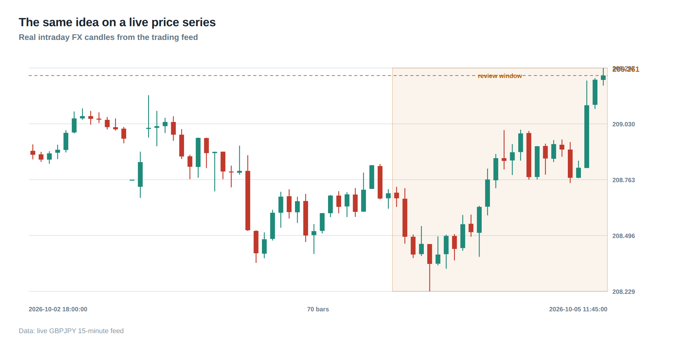
The mechanism described above assumes that volatility can be measured reliably from recent price history and that the market will continue to provide liquidity at the anticipated depth. In reality, several failure modes appear.

During a flash‑crash, price moves can be several standard deviations away from the recent mean within a few seconds, rendering the realised volatility estimate obsolete. The look‑back window, even if short, cannot anticipate such discontinuities, and the inverse‑volatility rule may still suggest a size that is too large for the instantaneous risk.

Another breakdown occurs when the market experiences a liquidity vacuum – for example, after a major economic announcement when many participants withdraw. The price impact function becomes highly non‑linear, and the assumed linear relationship between notional and P&L variance collapses. A position that would normally move one point per contract may now move five points per contract, inflating the realised loss far beyond the budget.

Execution‑related anomalies also undermine the model. Latency spikes, order‑stale events, and routing failures introduce tail delays that are not captured by the volatility estimate. When an order is delayed, the price may have moved several ticks, effectively increasing the realised volatility of the trade. The risk model, which only incorporates price variance, will miss this component, leading to an under‑estimation of the true exposure.

Finally, structural changes such as a shift from a continuous auction to a call‑auction regime alter the statistical properties of returns. The historical distribution used for the estimate no longer represents the future distribution, and the scaling rule becomes mis‑aligned with the new market micro‑structure.

The operating path, stage by stage

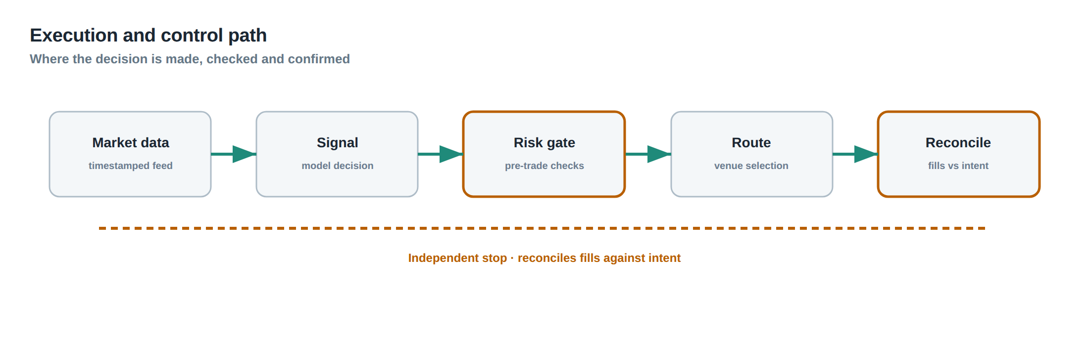
The live system follows a deterministic pipeline that begins with data ingestion and ends with trade execution, with risk controls interleaved. First, the market data feed supplies tick‑by‑tick prices, from which the engine aggregates 5‑minute bars. These bars feed a rolling window that computes the realised standard deviation, updating the volatility estimate each minute.

Second, the risk engine receives the latest estimate and the pre‑defined risk budget, applying the inverse‑volatility formula to generate a raw target notional. At this point the floor and cap module checks the raw size against the minimum and maximum contract limits, truncating where necessary.

Third, the market‑state monitor evaluates a set of qualitative signals: recent order‑book depth, trade‑through frequency, and any active market halts. If any flag crosses a threshold, the discretionary reduction factor is applied, further scaling down the target notional.

Fourth, the order manager translates the final contract count into a set of limit or market orders, respecting the venue‑specific maximum order size and the desk’s internal turnover ceiling. The orders are then routed through the preferred gateway, with a fallback path ready in case of connectivity loss.

Finally, after execution, the P&L calculator records the realised profit, the slippage, and the realised volatility of the trade. These figures are fed back into the performance logger, which updates the rolling risk statistics used for the next iteration of the pipeline. The entire loop repeats every minute, ensuring that the exposure remains aligned with the most recent market conditions.

Controls that act before the damage

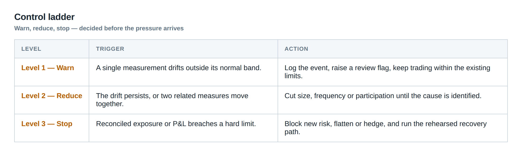
Preventative controls are placed at each decision node to avoid the escalation of risk. The first line of defence is the volatility‑estimation sanity check: if the computed standard deviation exceeds a pre‑set multiple of the historical median (for example, 3 × median), the estimate is flagged as an outlier and replaced by the median value for that instrument. This caps the influence of extreme spikes on the size calculation.

The second control is the floor‑and‑cap module, which guarantees that the algorithm never exceeds the desk’s market‑impact budget. The floor also prevents the algorithm from shrinking to a size where fixed transaction costs dominate, thereby preserving economic viability.

A third layer is the market‑state filter, which monitors order‑book imbalance, spread widening, and the frequency of stale quotes. When the spread widens beyond a threshold (e.g., 5 ticks) or the stale‑order rate exceeds 2 % of total orders in the last 30 seconds, the filter triggers a reduction factor of 0.5. This pre‑emptive shrinkage reduces exposure before the market deteriorates further.

The fourth safeguard is the execution‑quality monitor. It records latency distributions and the proportion of orders that are cancelled before execution. If the 95 th‑percentile latency exceeds a hard limit (for instance, 200 ms), the system automatically suspends new order submission for that instrument until latency returns to acceptable levels.

Together these controls form a ladder that catches risk‑inflating conditions at the earliest possible stage, ensuring that the size‑adjustment rule never operates on corrupted inputs.

How to measure whether it is working

Effectiveness is assessed by comparing the realised risk of each trade to the pre‑trade budget. The primary metric is the realised one‑sigma loss, calculated as the absolute P&L divided by the realised standard deviation of the trade’s price path. If the average realised loss consistently stays below the allocated budget, the scaling rule is functioning as intended.

A secondary metric is turnover‑adjusted Sharpe ratio, which incorporates the cost of re‑sizing. Because the volatility‑based rule can generate frequent size changes, the net P&L after transaction costs must be examined. A decline in this ratio indicates that the look‑back window may be too short, producing noisy estimates and excessive re‑balancing.

The third diagnostic is the breach frequency: the proportion of trades where realised loss exceeds the budget by more than a factor of two. A low breach frequency (under 5 %) suggests that the floor‑and‑cap and market‑state filters are successfully containing tail events.

Finally, a regression of realised loss against the volatility estimate can reveal systematic bias. A slope significantly different from one indicates that the estimate either under‑ or over‑states the true risk, prompting a recalibration of the look‑back period or the scaling constant.

These quantitative checks are run daily, with alerts generated when any metric drifts beyond pre‑defined control limits. The alerts trigger a review of the parameter set and, if necessary, a temporary suspension of the strategy.

The portfolio view

When the volatility‑scaled sizing rule is applied across a basket of instruments, the portfolio’s aggregate risk becomes more stable than the sum of its parts. Each instrument contributes a risk amount that is normalised to the same budget, so the portfolio’s variance is the sum of the individual budgets plus a modest covariance term.

Because the rule automatically reduces exposure in turbulent markets, the portfolio’s overall VaR tends to be less sensitive to market regime shifts. During a market‑wide volatility surge, many positions shrink simultaneously, dampening the aggregate tail. Conversely, in a low‑volatility environment, the caps prevent the portfolio from ballooning to an unmanageable size, preserving liquidity and limiting market impact.

The portfolio‑level risk manager can therefore set a single capital‑allocation target – for example, 2 % of equity at risk across all strategies – and rely on the per‑instrument volatility scaling to enforce that target dynamically. The manager still monitors the net turnover, as excessive re‑sizing across many instruments can erode net returns.

A holistic view also requires tracking the realised correlation between instruments during stress periods. If correlations spike, the aggregate risk may exceed the simple sum of individual budgets. In that case, an additional portfolio‑level cap can be imposed, scaling down all positions proportionally when a stress‑correlation threshold is breached.

In practice, the combination of per‑instrument volatility scaling, disciplined floor/cap limits, and a portfolio‑wide stress filter yields a risk profile that is both responsive and bounded, aligning the desk’s capital utilisation with its risk appetite across all market regimes.

Do you think your current position‑sizing framework adequately reflects the volatility dynamics of the instruments you trade?

About the research behind this lesson

Andrew Lo's lectures build risk analysis from return distributions and statistical measures, rather than treating one realised result as a complete description of risk.

Applied to this lesson: For a fast strategy, median latency or average fill quality is not enough. The review has to include tail delays, stale-order frequency and the loss distribution when cancellation or routing behaves abnormally.

Explore PULSE: System details

PULSE live account: Verify the live account on FX Blue

Live chat and updates: Telegram @xtrskhft

Source: Risk and Return

Educational content only. Trading leveraged products involves risk.