October 29, 2026

What this problem really is

Cross‑venue arbitrage is often described as “buy low on one exchange, sell high on another”. In practice the two displayed quotes are only the tip of a deep, dynamic order‑book. The moment a trader sends a marketable order to the cheap venue, the best offer may already be gone, and the price that was printed a few milliseconds earlier may have moved. Moreover, the two legs of the trade are bound by the rules of each venue – settlement cycles, margin requirements, and the ability to move inventory in real time. If the venue that offers the lower price cannot release the position quickly enough, the arbitrageist is forced to hold the asset on the cheap side while waiting for the expensive side to clear, exposing the desk to funding costs, withdrawal limits and, in extreme cases, a complete inability to close the position. The core thesis is therefore that a price gap on the screen is not an executable arbitrage unless the surrounding ecosystem – inventory, settlement, fees and venue‑specific constraints – permits both legs to be completed within the window that the gap persists.

The literature on electronic markets models each venue as a price‑time priority queue. The value of a queue position can be split into three components: the expected spread capture, the adverse‑selection cost of being front‑run, and the option‑value of retaining a place in line for a future favourable move. When a trader evaluates a cross‑venue opportunity, the decision to keep an order alive cannot be based on elapsed clock time alone; it must be refreshed continuously against the evolving queue value, the anticipated fee structure and the probability that the opposing venue will still have depth when the order reaches the market.

Consequently, the problem is not simply “spot the price difference”, but “manage a pair of contingent executions that respect the micro‑structure of two independent markets”. The desk must therefore treat each leg as a conditional order, with explicit constraints on inventory transfer speed, funding availability and the risk that one side may be forced to unwind at an unfavourable price if the other side fails to execute.

How the mechanism works, step by step

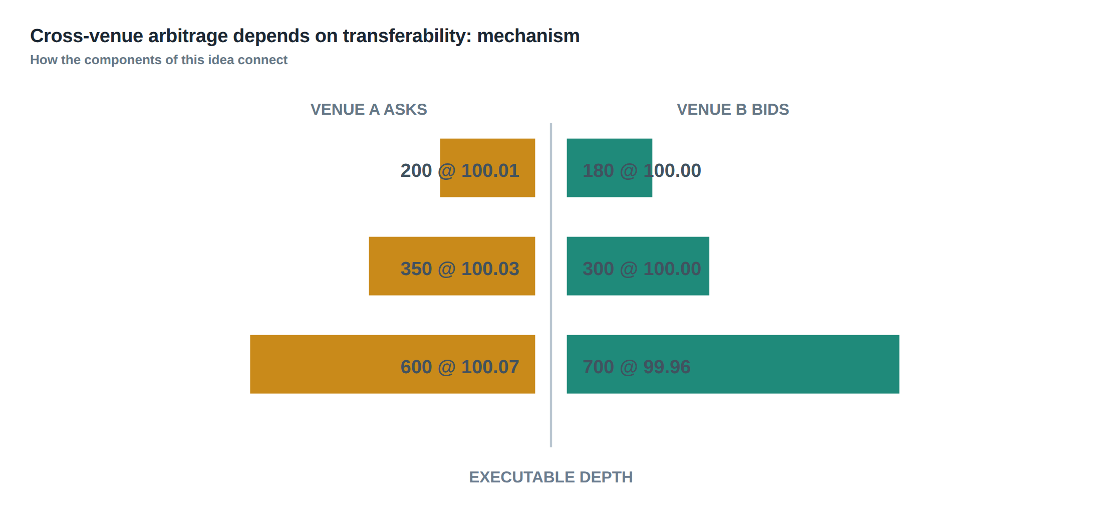
The first step is to monitor the top‑of‑book and the depth of both venues in real time. A genuine arbitrage signal emerges only when the best bid on Venue A exceeds the best ask on Venue B after adjusting for all known transaction costs – exchange fees, clearing fees, and any rebates that may be earned by providing liquidity. The second step is to assess the execution horizon: how long does the observed spread need to survive for the pair of orders to be filled? This horizon is a function of the average order‑book turnover on each side, the latency of the order‑routing infrastructure, and the expected latency of inventory transfer, which may be limited by settlement cycles (T+0 versus T+2) or by internal credit lines between the two venues.

If the transfer time exceeds the expected lifespan of the spread, the desk must pre‑position inventory. Pre‑positioning means holding a net long or short exposure on the venue that will later provide the opposite leg, funded either by internal capital or by borrowing against collateral. The decision to pre‑position is itself an optimisation problem: the cost of funding the inventory (interest on cash or the hair‑cut on borrowed securities) must be weighed against the expected arbitrage profit after fees.

The third step is to submit the two orders as contingent or “fill‑or‑kill” pairs. Many execution platforms allow a single logical order to be split across venues with a dependency flag – the sell order on Venue A will only be sent if the buy order on Venue B is confirmed, and vice‑versa. This reduces the exposure to one‑sided execution but introduces a new risk: if one venue experiences a temporary outage, the dependent order may sit in the queue indefinitely, accruing adverse‑selection costs and potentially violating inventory limits.

Finally, the desk must monitor the post‑trade state. Settlement messages from each venue confirm whether the legs have cleared, and any residual inventory must be reconciled. If a leg fails, the desk must unwind the remaining exposure, often at a cost that erodes the original spread. The entire workflow is therefore a loop of detection, feasibility assessment, conditional execution, and post‑trade reconciliation, each stage governed by the micro‑structure constraints of the two markets.

A worked example with real numbers

Consider a futures contract that trades on Exchange X and Exchange Y. At 09:15:23 GMT the best ask on X is 12 500 USD, while the best bid on Y is 12 520 USD. The quoted spread is therefore 20 USD. Exchange X charges a taker fee of 0.015 % (≈ 1.88 USD on a 12 500 contract) and offers a maker rebate of 0.005 % (≈ 0.63 USD) if the order adds liquidity. Exchange Y levies a taker fee of 0.012 % (≈ 1.50 USD) and a maker rebate of 0.004 % (≈ 0.50 USD). The net fee to buy on X and sell on Y, assuming both orders are marketable, is 1.88 + 1.50 = 3.38 USD. Subtracting the 20 USD spread leaves a raw gross profit of 16.62 USD per contract.

However, the trader holds no inventory on X. The settlement system on X is T+0, but the internal transfer protocol to move the purchased contract to Y takes on average 150 ms, with a worst‑case of 300 ms during peak traffic. The observed spread on the two books historically survives for an average of 250 ms before converging. Because the transfer latency exceeds the median spread lifespan, the trader decides to pre‑position a short contract on Y, borrowing it against existing collateral. The borrowing cost is 0.02 % per hour, which for a 250 ms exposure is negligible (≈ 0.001 USD).

The trader submits a limit buy order on X at 12 500 USD with a fill‑or‑kill flag, and simultaneously a limit sell order on Y at 12 520 USD, also fill‑or‑kill. Both orders are routed through a low‑latency gateway that adds 30 ms of round‑trip time. The orders reach the markets at 09:15:23.150 GMT. The buy on X fills instantly; the sell on Y also fills, but only after the internal transfer of the borrowed contract completes at 09:15:23.300 GMT. The total realised profit, after fees, is 20 USD – 3.38 USD = 16.62 USD, less a negligible funding cost, confirming a successful arbitrage.

If the same gap appears but the transfer latency spikes to 400 ms because of a temporary network congestion, the sell order on Y would miss the top of the book, slipping to 12 515 USD. The spread would then be 15 USD, insufficient to cover the 3.38 USD fee, leaving a net loss of 1.38 USD. The example illustrates how the same printed price gap can either be a viable arbitrage or an unreachable illusion depending on the speed of inventory movement and the fee landscape.

Where it breaks in live markets

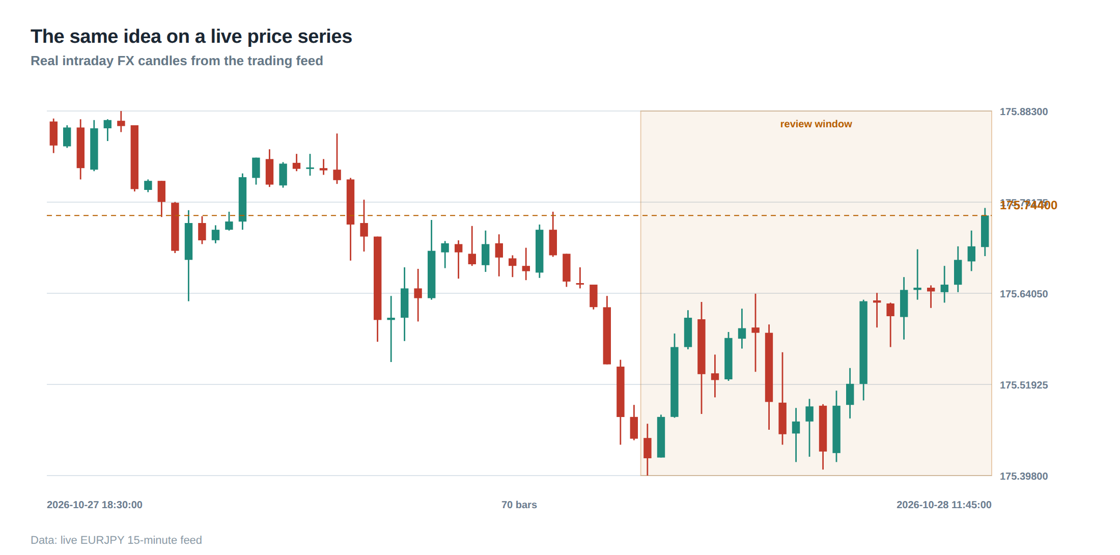
In a live environment the assumptions that underpin the example are constantly challenged. First, the depth of the order‑book can evaporate in a single millisecond when a large hidden order or a latency‑arbitrage bot sweeps the level, turning a visible 20 USD spread into a 0 USD spread before the trader’s order arrives. Second, venue‑specific settlement rules can impose mandatory waiting periods; some dark pools settle on a delayed net‑ting schedule that can be hours long, making any cross‑venue pair that relies on immediate settlement impossible.

Third, fee structures are not static. During periods of high volume exchanges may adjust taker fees upward to manage load, while rebates may be withdrawn for certain order‑types. A trader who has hard‑coded the fee assumptions into the arb engine will see the expected profit evaporate, sometimes turning a marginally profitable trade into a loss. Fourth, funding constraints can appear abruptly. If the desk’s cash balance on a venue falls below the required margin because of an unrelated position, the system may reject the new order, leaving the opposite leg exposed.

Finally, venue outages, whether planned maintenance or unexpected crashes, break the dependency chain. If Exchange Y suffers a brief disconnect after the buy on X has been executed, the sell order cannot be sent, and the desk is left holding a long position that must be unwound on X at a later, possibly adverse price. Counter‑party exposure rises because the desk now owes the borrowed contract on Y without a corresponding offset, increasing the risk of margin calls.

The operating path, stage by stage

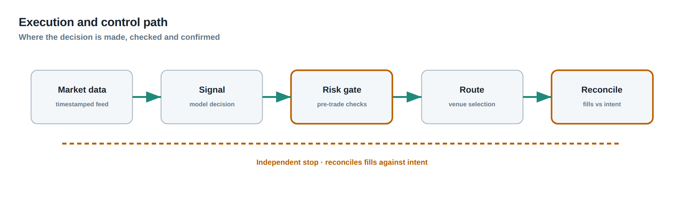
The first stage is market‑data ingestion. A high‑throughput feed handler normalises the depth snapshots from each venue, applies a fee schedule, and calculates the net spread after adjusting for expected rebates. The second stage is feasibility filtering, where the engine compares the net spread against a dynamic latency budget that incorporates current network latency, internal transfer times and the statistical survival distribution of the spread.

The third stage is inventory assessment. The system queries the position book for each venue, checks funding availability, and decides whether pre‑positioning is required. If pre‑positioning is needed, a separate funding order is generated, typically a cash transfer or a securities‑borrow request, and the engine waits for confirmation before proceeding.

The fourth stage is order generation. Conditional orders are built with explicit dependency flags – “execute sell on Y only if buy on X succeeds”. These orders are sent to a smart order router that selects the lowest‑latency path and adds a timestamp to aid post‑trade reconciliation.

The fifth stage is execution monitoring. A watchdog tracks acknowledgements, fills and any rejections. If a rejection occurs on one leg, the system automatically cancels the counterpart and initiates a unwind routine that respects the current market depth to minimise slippage.

The final stage is settlement verification. Settlement messages from each venue are matched against the internal ledger; any discrepancy triggers an exception workflow that may involve manual intervention. Throughout the pipeline, health‑checks and timeout thresholds are enforced to prevent the engine from persisting with stale orders when market conditions change.

Controls that act before the damage

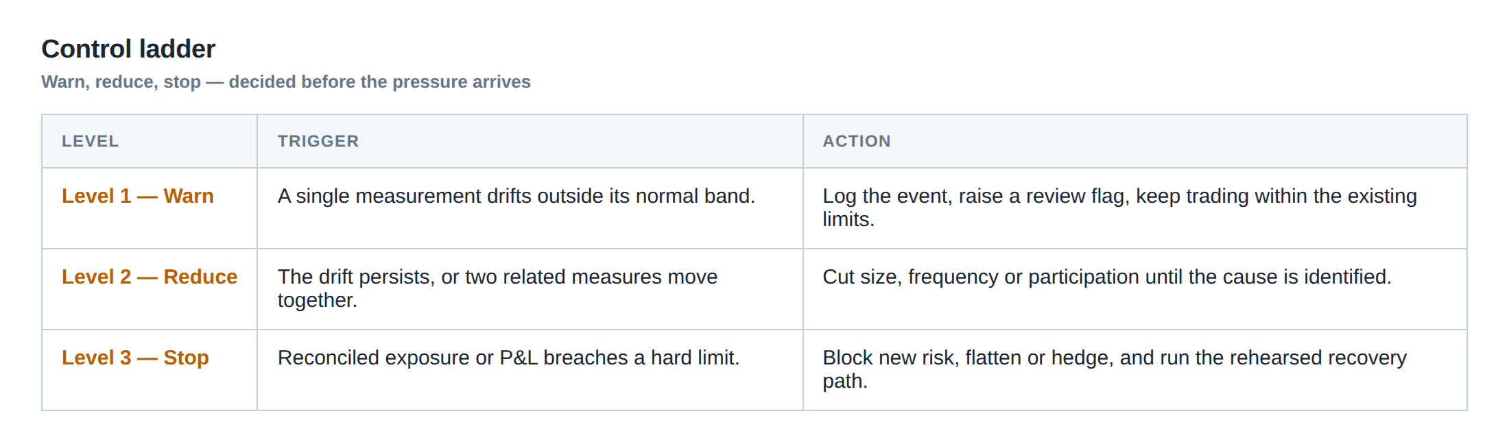
Preventive controls begin with a static latency model that is regularly calibrated against observed round‑trip times. The model defines a maximum acceptable latency for each venue pair; any arbitrage signal that would require a faster transfer is filtered out before reaching the order‑generation stage.

Dynamic fee validation is another guardrail. The system subscribes to fee‑change broadcasts from each exchange and recomputes the net spread in real time. If a fee increase pushes the expected profit below a pre‑set threshold, the signal is discarded.

Inventory buffers are maintained on each venue to absorb sudden funding shortfalls. The desk sets a minimum cash and securities cushion – for example, a 5 % excess of the maximum notional that could be tied up in a single arbitrage – and the engine refuses to launch a trade that would breach the buffer.

A pre‑trade credit‑limit check ensures that any borrowing required for pre‑positioning does not exceed the counter‑party’s approved limit. If the limit is reached, the engine either reduces the trade size or aborts the attempt.

Finally, a simulated outage drill runs continuously in a sandbox environment. The engine injects artificial disconnects on one venue and verifies that the dependent order is cancelled within the prescribed timeout, that the unwind routine respects the current depth, and that no residual inventory is left hanging. These controls collectively reduce the probability that a printed spread becomes a source of loss.

How to measure whether it is working

The primary metric is the realised net profit per trade after all fees, funding costs and unwind losses. This figure should be compared against the theoretical profit calculated at the signal stage; the difference is the execution loss, which must stay within a tight band (typically less than 5 % of the gross spread).

A secondary measure is the fill‑rate of the dependent leg. The ratio of successful paired executions to total attempted pairs indicates how often the latency and inventory constraints are being respected. A declining fill‑rate signals degradation in either network performance or venue reliability.

The third indicator is the average time‑to‑settlement for each leg. If settlement times creep upward, the pre‑positioning buffer may need to be enlarged, or the latency budget tightened.

Lastly, the frequency of forced unwind events – situations where one leg fills and the other does not – should be tracked. A low unwind frequency, coupled with a small average unwind loss, demonstrates that the contingency logic and the outage controls are effective. Continuous monitoring of these statistics, plotted on rolling windows, provides early warning of emerging weaknesses.

The portfolio view

From a portfolio perspective, cross‑venue arbitrage is a micro‑structure overlay that sits alongside directional, statistical and macro‑factor exposures. It contributes a near‑zero‑beta return stream, but its risk profile is highly asymmetric: the upside is capped by the spread, while the downside can be amplified by funding costs, margin calls or forced unwind losses.

Because each arbitrage leg ties up capital on two distinct venues, the desk must allocate capital buffers that respect the aggregate exposure across all active pairs. The net‑cash position on each venue should be monitored to avoid unintended net long or short bias that could interfere with other strategies.

Correlation between arbitrage opportunities and market volatility is typically low, but during periods of extreme stress (e.g., flash crashes) the price gaps can widen dramatically, tempting the desk to increase size. At the same time, latency spikes and settlement delays become more common, raising the probability of a one‑sided fill. Hence, the risk‑management framework must dynamically scale the maximum allowable notional based on real‑time latency and outage metrics, not merely on historical volatility.

In practice, the arbitrage desk reports its performance as a separate sub‑portfolio, with its own risk‑adjusted return metrics (Sharpe, Sortino) and its own limits on gross exposure, inventory turnover, and drawdown. This segregation allows senior management to assess whether the cross‑venue activity is delivering the intended low‑correlation alpha without contaminating the risk profile of the broader trading book.

Do you have a systematic way of testing whether your inventory‑transfer latency can keep pace with the fleeting spreads you target?

About the research behind this lesson

The seminar frames electronic markets as price-time-priority queues. It separates queue value into spread capture versus adverse-selection cost and the option value of retaining a place in line.

Applied to this lesson: An order lifetime therefore cannot be based on elapsed time alone: the system must reassess whether its queue position, expected spread and adverse-selection risk still justify keeping the order alive.

Two live systems, one desk

PULSE-X — power-packed HFT: high-frequency momentum on XAUUSD and EURUSD. System details · Live account

NIC-X — ultra-low drawdown: displaced-print arbitrage for large capital. System details · Live account

Start now: leave your email and request a free trial — we will send the pricing, the connection route and the trial terms. Pricing

Live chat and updates: Telegram @xtrskhft

Source: High-Frequency Trading and Modern Market Microstructure

Educational content only. Trading leveraged products involves risk.