October 29, 2026

What this problem really is

When a trader quotes a stop loss, the price distance from entry to stop is often taken as a proxy for the amount of capital that could be lost. In reality the distance alone tells nothing about the monetary exposure because the exposure is a product of three variables: the size of the position, the contract specifications of the instrument, and the currency in which the profit‑and‑loss is settled. Ignoring any of these components turns a purely geometric notion of risk into a misleading figure that can easily breach a firm’s risk budget.

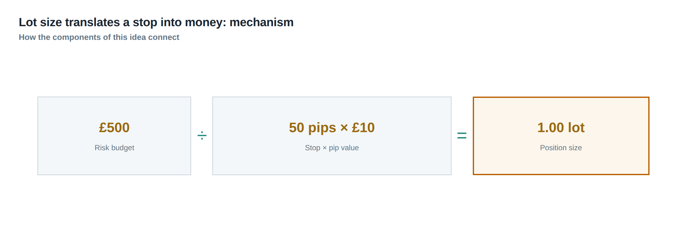
A disciplined prop‑trading desk therefore begins every trade idea with an explicit risk budget – for example a £500 maximum loss on a single position. This figure is absolute, not relative, and it is the ceiling that the combination of stop distance, contract size and lot increment must respect. All subsequent calculations are anchored to this budget; if the stop moves, the contract size changes, or the tick value is altered, the position size must be recomputed to keep the monetary risk within the prescribed limit.

The mistake of treating stop distance as the sole determinant of risk is amplified when the instrument trades in a different currency or when the venue imposes a minimum lot size that is larger than the mathematically exact solution. In such cases the trader must round down to the nearest permissible lot, which inevitably reduces the theoretical exposure and introduces a buffer – but only if the rounding is performed deliberately and not as an after‑thought.

How the mechanism works, step by step

First, the trader translates the stop distance measured in price units into a number of ticks. A tick is the smallest price increment recognised by the exchange; its monetary value is fixed by the contract specifications. For a futures contract on the FTSE 100, for instance, one tick equals 0.5 index points and is worth £10. Multiplying the number of ticks by the tick value yields the profit‑and‑loss per contract for a full‑stop move.

Second, the trader determines how many contracts can be held before the loss on a full‑stop move reaches the risk budget. This is simply the risk budget divided by the per‑contract loss. Because the venue only allows integer multiples of a base lot – often one contract or a defined fraction such as 0.5 lots – the raw contract count is rounded down to the nearest allowable increment. The rounding step guarantees that the actual monetary exposure never exceeds the budget, even if the stop is hit exactly.

Third, the trader adds the expected cost of execution. The spread is the immediate price concession that must be paid to cross the bid‑ask, and slippage represents the additional adverse movement that can occur between order submission and fill. Both are expressed in ticks and are subtracted from the theoretical profit‑and‑loss per contract before the position size is finalised. The final position size therefore reflects the true amount of capital that could be lost after accounting for all known transaction costs.

A worked example with real numbers

Assume a trader has a £500 risk budget for a single trade on the E‑mini S&P 500 futures (ticker ES). The contract size is one futures contract representing $50 per index point, and the tick size is 0.25 points, each tick worth $12.50. The trader’s account base currency is pounds, and the current USD/GBP rate is 0.78, giving a tick value of £9.75.

The entry price is 4 200 points and the stop is placed 40 points away, i.e. 160 ticks. The raw loss per contract if the stop is hit is 160 ticks × £9.75 = £1 560. Dividing the £500 risk budget by £1 560 yields 0.32 contracts. The venue’s minimum lot increment is 0.1 of a contract, so the trader rounds down to 0.3 contracts. Before execution the trader expects a spread of two ticks (£19.50) and an average slippage of three ticks (£29.25). The total cost per contract is therefore £48.75, which reduces the effective loss per contract to £1 511.25. Re‑calculating the allowable contracts with the cost‑adjusted loss gives £500 / £1 511.25 ≈ 0.33, which again rounds down to 0.3 contracts.

Now consider a stop that is twice as wide – 80 points or 320 ticks. The raw loss per contract doubles to £3 120. The same £500 budget now permits only 0.16 contracts; rounding down to the nearest 0.1 lot yields 0.1 contracts. After adding the same spread and slippage (now proportionally larger because the stop is wider, but we keep the same expected values for illustration), the effective loss per contract is roughly £3 071, and the permissible size remains 0.1 contracts. In effect, doubling the stop distance halves the position size before costs, confirming the core thesis that distance alone does not set risk – it is the interaction with contract size and cost that does.

Where it breaks in live markets

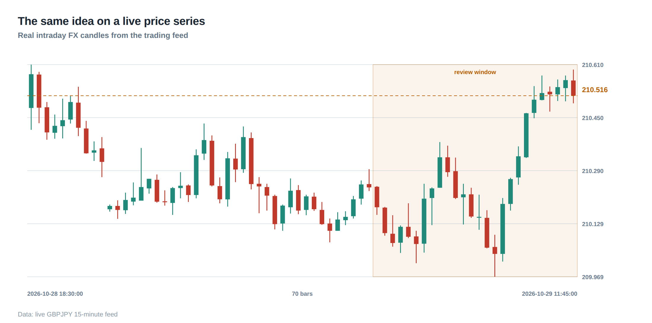
The tidy arithmetic above assumes that the market will honour the quoted tick value and that the spread and slippage are predictable. In reality, high‑frequency moves, order‑book gaps, or sudden news releases can cause the execution price to deviate dramatically from the theoretical level. When volatility spikes, the stop may be triggered several ticks beyond the intended level, a phenomenon known as slippage explosion. If the trader has not built a buffer for such tail events, the realised loss can exceed the risk budget despite having followed the calculation correctly.

Another source of breakdown is the latency of the order routing chain. A median latency of, say, 2 ms may look acceptable, but the distribution often has a heavy right tail; occasional latency outliers of 20 ms or more can cause the stop order to be placed after the market has already moved past the intended price. The loss distribution therefore acquires a fat tail that is not captured by the simple spread‑plus‑slippage estimate.

Finally, the assumption of a static currency conversion rate can be violated in cross‑currency futures. If the GBP depreciates sharply against the USD between entry and exit, the pound‑denominated loss per tick rises, inflating the monetary exposure. Without a dynamic conversion adjustment, the risk budget can be breached without any change in the underlying price movement.

The operating path, stage by stage

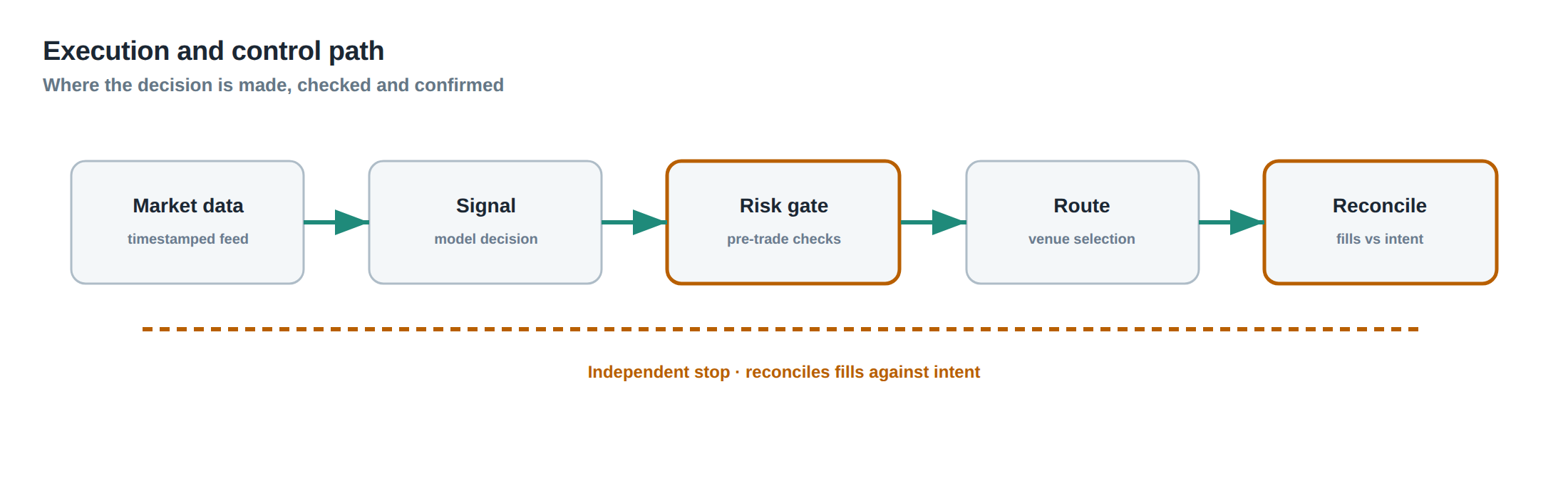
The first stage is risk budgeting, where the desk defines the maximum permissible loss per trade and per day. This figure is stored in the order‑management system (OMS) and is referenced for every new ticket. The second stage is stop‑distance translation, where the OMS queries the contract specifications – tick size, tick value, and currency – and computes the raw loss per contract. The third stage is lot‑size quantisation, where the raw contract count is rounded down to the nearest venue‑allowed increment, ensuring compliance with exchange rules.

The fourth stage incorporates execution costs. The OMS retrieves the current bid‑ask spread from the market data feed and applies a slippage model that may be based on recent order‑book depth or on a statistical estimate derived from historical fill data. The fifth stage is final position sizing, where the adjusted loss per contract is divided into the risk budget to obtain the maximum allowable contracts, which are then truncated to the lot increment. The sixth and final stage is order submission, where the calculated lot size, entry price, and stop price are sent to the gateway for routing.

At each transition, the system logs the intermediate values – raw loss, rounded contracts, cost adjustments – to provide a traceable audit trail. If any stage fails to produce a feasible lot size (for example, when the rounded lot would be zero), the OMS aborts the ticket and raises a warning to the trader.

Controls that act before the damage

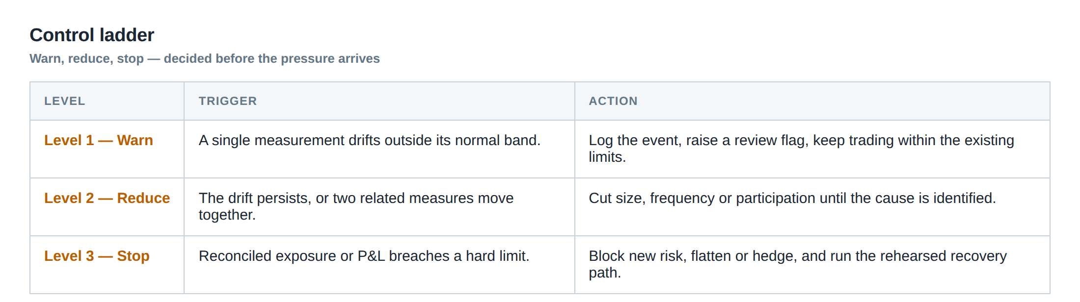
A robust control framework places safeguards at the points where the calculation could be corrupted. The first control is a pre‑trade limit check that validates the risk budget against the proposed position size; any breach triggers an automatic reduction of the lot size or a rejection of the order. The second control monitors real‑time spread and slippage estimates; if the observed spread widens beyond a pre‑set threshold, the system recalculates the lot size on the fly and may delay order transmission until conditions improve.

The third control is a volatility guard. The OMS continuously computes the realised volatility over the last N bars and, if the volatility exceeds a multiple of the historical average, it forces a re‑evaluation of the stop distance. Because the stop distance directly influences the raw loss per contract, a widening volatility environment typically leads to a reduction in position size to keep the monetary risk bounded.

The fourth control is a currency‑exposure hedge. When the instrument settles in a foreign currency, the system checks the current FX rate against a moving average; a deviation beyond a tolerance band prompts an automatic adjustment of the risk budget in the local currency, ensuring that the pound‑denominated exposure remains within the intended limit.

All these controls are implemented as deterministic rules within the OMS, and each rule produces a log entry that can be audited post‑mortem. By intervening before the order reaches the exchange, the desk can prevent a cascade of losses that would otherwise arise from a mis‑sized position.

How to measure whether it is working

Effectiveness is measured by comparing the realised loss distribution against the theoretical one generated by the pre‑trade calculations. The key metric is the proportion of trades where the absolute loss exceeded the risk budget; a well‑tuned system should keep this figure close to zero, acknowledging that occasional outliers are inevitable due to extreme market events.

Another indicator is the average utilisation of the risk budget. If the majority of trades consume only a small fraction of the £500 limit, the desk may be overly conservative, leaving capital idle. Conversely, if the average utilisation hovers near the limit but the breach rate remains low, the sizing algorithm is operating at an efficient frontier.

A third measurement involves the latency tail. By recording the time between stop order generation and fill, the desk can construct a latency distribution and verify that the 95th percentile remains within the expected envelope. An increase in the tail suggests that the slippage model may be under‑estimating execution risk, prompting a recalibration of the cost component in the sizing formula.

The portfolio view

When multiple strategies share the same capital pool, the individual risk budgets must be aggregated to respect an overall portfolio VaR or expected shortfall limit. Because each strategy may trade different instruments with varying tick values and currency exposures, the translation of stop distances into monetary risk must be performed on a per‑strategy basis before being summed.

The portfolio manager therefore monitors the cumulative risk consumption in real time, ensuring that the sum of the individual £500 allocations does not exceed the total risk ceiling – for example £5 000 for ten concurrent positions. If a strategy widens its stop due to a change in market volatility, the system automatically reduces its position size, freeing capacity for other desks to increase exposure elsewhere, provided the total risk budget remains intact.

Finally, the portfolio view must incorporate correlation effects. Two positions with stops that are likely to be triggered simultaneously – such as long and short contracts on highly correlated indices – can amplify the realised loss beyond the simple sum of their individual risk budgets. Stress‑testing the portfolio under joint stop‑out scenarios allows the desk to apply a correlation multiplier to the individual budgets, preserving the integrity of the overall risk framework.

Do you currently verify that every stop‑loss calculation on your desk incorporates contract specifications, spread, slippage and lot‑size rounding before committing capital?

About the research behind this lesson

Andrew Lo's lectures build risk analysis from return distributions and statistical measures, rather than treating one realised result as a complete description of risk.

Applied to this lesson: For a fast strategy, median latency or average fill quality is not enough. The review has to include tail delays, stale-order frequency and the loss distribution when cancellation or routing behaves abnormally.

Two live systems, one desk

PULSE-X — power-packed HFT: high-frequency momentum on XAUUSD and EURUSD. System details · Live account

NIC-X — ultra-low drawdown: displaced-print arbitrage for large capital. System details · Live account

Start now: leave your email and request a free trial — we will send the pricing, the connection route and the trial terms. Pricing

Live chat and updates: Telegram @squawklive_news

Source: Risk and Return

Educational content only. Trading leveraged products involves risk.