October 30, 2026

What this problem really is

The phrase “one lot” is often taken for granted as a constant measure of exposure – a single contract, a fixed notional, a static unit of risk. In practice the market’s intrinsic volatility is anything but static. When the typical price swing of the underlying widens, the same lot now represents a larger absolute move in the portfolio’s equity curve; when volatility contracts, the lot becomes comparatively inert. The mismatch between a fixed quantity and a fluid volatility environment creates an unstable risk profile that can erode capital during periods of heightened turbulence and leave capital idle when markets are calm.

The instability is not merely a theoretical curiosity. A prop‑trading desk that allocates a fixed number of contracts to a mean‑reversion strategy may see its daily P&L variance double overnight after a macro news release, even though the strategy’s logic has not changed. The underlying risk budget – the maximum acceptable standard deviation of returns – is therefore breached without any explicit signal. The core problem is that a static lot size decouples exposure from the statistical property that should drive it: the expected magnitude of price movement.

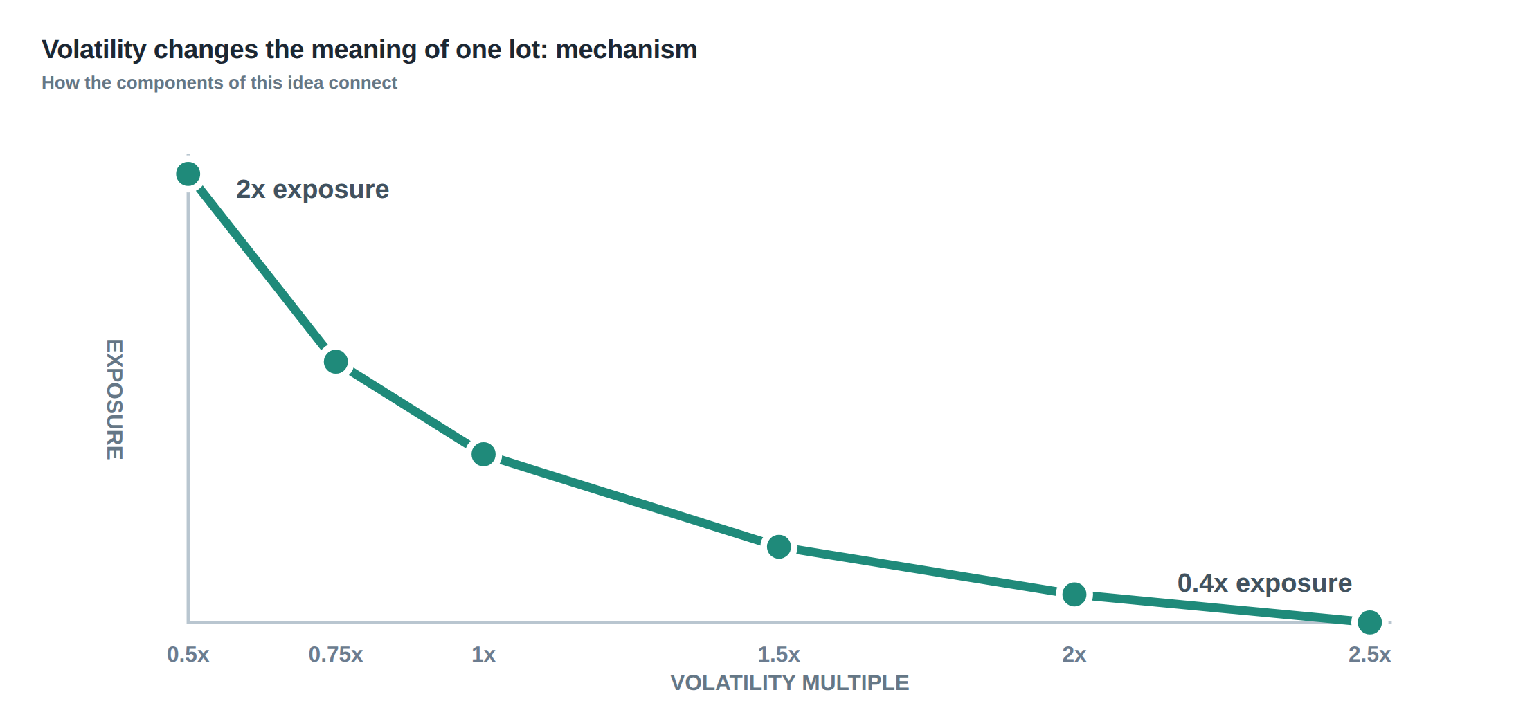
In quantitative terms, if we denote the risk budget as σ\_budget and the estimated daily volatility of the instrument as σ̂, a static lot size L yields an implied risk of L·σ̂. When σ̂ fluctuates, the implied risk fluctuates in direct proportion. The desk either over‑leverages during spikes or under‑leverages during lulls, both of which are undesirable. The solution is to let the lot size be a function of the volatility estimate, thereby preserving a stable proportion of the risk budget irrespective of market regime.

How the mechanism works, step by step

The first step is to obtain a volatility estimate that reflects the recent behaviour of the instrument. This is usually achieved with an exponentially weighted moving standard deviation or a GARCH‑type model applied to a chosen look‑back window. The look‑back length is a trade‑off: a short window reacts quickly to regime changes but introduces noise, while a long window smooths the estimate but lags behind abrupt shifts.

Once σ̂ is calculated, the desk defines a target exposure factor κ such that the product κ·σ̂ equals the pre‑agreed risk budget σ\_budget. Rearranging gives κ = σ\_budget / σ̂, which is the scaling factor applied to the base lot size. The actual number of contracts N is then N = κ·L\_base, where L\_base is the nominal lot that would be used if volatility were at a reference level σ\_ref.

To prevent the scaling factor from exploding during extreme volatility spikes or collapsing to zero when markets freeze, floors and caps are imposed on κ. A lower bound ensures a minimum level of market participation, while an upper bound caps the maximum exposure, protecting the desk from allocating an unmanageable number of contracts.

Finally, the desk monitors market conditions for signs of discontinuity – such as trading halts, wide bid‑ask spreads, or abnormal order‑book depth. In those circumstances the volatility estimate may be unreliable, and the scaling rule is temporarily suspended or further constrained, reducing exposure until normal conditions resume.

A worked example with real numbers

Assume a statistical arbitrage strategy that normally trades 50 contracts of a futures contract when volatility is at its historical average of 1.2 % per day. The desk’s risk budget is set at a daily volatility exposure of 0.6 % of equity. With the reference volatility σ\_ref = 1.2 % and base lot L\_base = 50, the implied risk at the reference point is 50 × 1.2 % = 60 % of the daily volatility budget, meaning the scaling factor κ\_ref = σ\_budget / σ\_ref = 0.6 % / 1.2 % = 0.5. Consequently the base exposure is already half of the maximum allowed, leaving headroom for volatility increases.

Now suppose a sudden macro event pushes the realised volatility estimate to σ̂ = 2.4 % – exactly double the reference. The inverse‑volatility rule dictates κ = 0.6 % / 2.4 % = 0.25. Applying this to the base lot yields N = 0.25 × 50 = 12.5 contracts, which the desk rounds to 12 contracts. In effect, the exposure is halved relative to the original 25‑contract position that would have been used if the volatility had remained at 1.2 %. The risk contribution of the position stays at the prescribed 0.6 % of equity despite the doubled price swing.

If volatility were to fall to 0.6 % – half the reference – the scaling factor rises to κ = 0.6 % / 0.6 % = 1.0, and the desk would trade the full 50 contracts, thereby utilising the entire risk budget. Should the estimate dip further to 0.3 %, the uncapped rule would suggest κ = 2.0, implying 100 contracts, but a pre‑defined cap of κ\_max = 1.5 would limit the position to 75 contracts, protecting the desk from over‑concentration in a low‑volatility, potentially illiquid environment.

The example illustrates the direct arithmetic relationship: a doubling of the volatility estimate, with an unchanged risk budget, leads to a halving of the contract count. The same logic applies symmetrically in the opposite direction, moderated by the caps and floors that the desk has chosen.

Where it breaks in live markets

The volatility‑scaled lot methodology presumes that the volatility estimate is a reliable proxy for future price movement. In reality, markets can experience discontinuities that invalidate the estimate. Sudden order‑book imbalances, flash crashes, or algorithmic cascades can generate price moves that are orders of magnitude larger than the recent statistical history. In such cases, the scaling rule may still produce a position that, while mathematically within the risk budget, is exposed to execution risk far beyond the model’s assumptions.

Another failure mode is the latency of the volatility feed. If the estimate is derived from a data source that lags the exchange by several seconds, the scaling factor will be based on stale information. During high‑frequency bursts, the actual realised volatility can outpace the estimate, causing the desk to be over‑leveraged for a brief but potentially damaging interval.

Liquidity also plays a decisive role. When volatility spikes, market depth often evaporates, and the cost of entering or exiting the scaled position can exceed the theoretical risk budget. The model does not automatically account for widening spreads or the probability of partial fills, which can turn a modest position into a sizeable slippage loss.

Finally, the presence of regime‑switching behaviour – for example, a transition from a mean‑reverting to a trending market – can render a volatility‑only scaling rule insufficient. The risk profile of the strategy may change qualitatively, and the same exposure level that was appropriate under one regime may become inappropriate under another, leading to systematic under‑performance or unexpected drawdowns.

The operating path, stage by stage

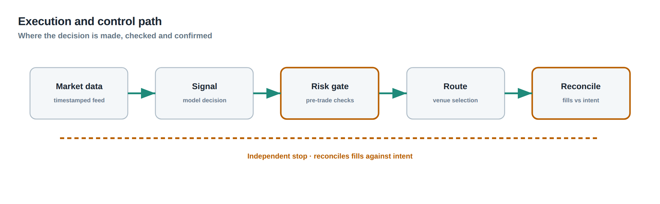
The first stage is data acquisition: high‑frequency price series are ingested, cleaned, and normalised. From this stream the desk computes a realised return series, typically using log‑returns over a fixed interval such as one minute. The second stage is volatility estimation, where an exponentially weighted moving standard deviation is applied to the return series over a look‑back window that the desk has calibrated to balance responsiveness against statistical noise.

The third stage translates the volatility estimate into a scaling factor. The desk divides the pre‑agreed risk budget by the estimated volatility, then applies any pre‑set caps and floors to the resulting factor. The fourth stage converts the capped scaling factor into an integer contract count, rounding according to the market’s minimum trade size and any position‑sizing constraints such as maximum per‑instrument exposure.

The fifth stage is order generation. The desk builds a set of limit or market orders that reflect the desired contract count, while also incorporating execution policies that limit market impact – for example, slicing the order across multiple price levels or time slices. The final stage is post‑trade monitoring: realised P&L, slippage, and the realised volatility of the executed trades are recorded, feeding back into the next estimation cycle.

Each stage contains decision points that can be overridden by risk controls. For instance, if the order‑book depth falls below a threshold, the order generation stage may be halted, or the scaling factor may be temporarily reduced. This staged architecture ensures that the volatility‑scaled exposure is continuously reconciled with the live market environment.

Controls that act before the damage

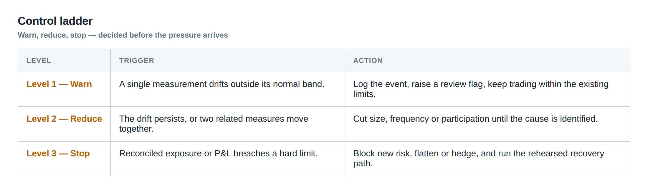
Before a position is taken, the desk applies a hierarchy of safeguards. The first line of defence is the volatility‑cap filter: if the estimated volatility exceeds a pre‑determined maximum, the scaling factor is forced to the upper cap, thereby limiting the absolute number of contracts. The second line is the liquidity guard, which checks the current order‑book depth and the average daily volume of the instrument; if the depth falls below a multiple of the intended trade size, the desk either reduces the contract count or aborts the trade entirely.

A third safeguard is the execution‑quality monitor. It tracks the latency distribution of recent order acknowledgements and the frequency of stale‑order rejections. When tail latencies breach a threshold, the desk temporarily switches to a more conservative scaling regime, effectively lowering κ until the latency profile normalises.

The fourth control is the regime‑detection module. By analysing higher‑order moments of the return distribution – skewness, kurtosis, and the frequency of extreme moves – the module flags periods where the market is behaving in a non‑Gaussian fashion. In such periods the desk may impose an additional multiplicative reduction on the scaling factor, ensuring that the exposure does not rely solely on the standard deviation estimate.

Finally, a manual oversight checkpoint exists for instruments that have recently undergone corporate actions, exchange rule changes, or have been subject to regulatory halts. In those cases, the automated volatility estimate is ignored and a discretionary exposure limit is applied until the data stream stabilises.

How to measure whether it is working

The primary metric is the realised volatility of the scaled position relative to the risk budget. After each trading day the desk computes the standard deviation of the strategy’s returns, weighted by the actual contract counts used, and compares it with the target σ\_budget. A ratio close to one indicates that the scaling rule is preserving the intended risk level.

A secondary measure is the tracking error between the predicted volatility (the σ̂ used to set the size) and the realised volatility of the instrument over the same horizon. Persistent under‑estimation suggests that the look‑back window is too short or that the model is missing structural changes, while chronic over‑estimation may indicate that the caps are overly restrictive.

Execution performance is also monitored. The average slippage per contract, the proportion of orders filled at the quoted price, and the incidence of partial fills are all recorded. If slippage consistently erodes more than a pre‑defined fraction of the risk budget, the desk must tighten the liquidity guard or adjust the caps.

Finally, the desk examines the distribution of daily P&L contributions from the volatility‑scaled component. A well‑behaved system should produce a near‑Gaussian distribution centred around zero, with tail losses that are within the expected confidence interval derived from the risk budget. Deviations from this pattern trigger a review of the scaling parameters and the underlying volatility estimator.

The portfolio view

When each instrument in a multi‑asset portfolio is sized according to its own volatility estimate, the aggregate risk becomes a function of the correlation matrix as well as the individual scalings. By normalising each position to the same proportion of its own risk budget, the desk ensures that no single market dominates the portfolio’s volatility, even if that market experiences a sudden surge.

However, the portfolio‑level volatility is not simply the sum of the individual variances; cross‑asset covariances must be accounted for. The desk therefore recomputes the portfolio’s expected variance after each scaling update, using the latest correlation estimates. If the portfolio variance exceeds a higher‑level risk ceiling, the desk may apply a second‑order scaling – reducing all positions proportionally – to bring the total risk back within limits.

This hierarchical approach allows the desk to maintain a stable risk profile both at the instrument level and at the portfolio level, despite the ever‑changing volatility landscape. It also facilitates capital allocation decisions: instruments with persistently low volatility can be given a larger nominal lot size without breaching the overall risk ceiling, while high‑volatility instruments are automatically throttled.

The ultimate benefit is a risk‑aware exposure framework that adapts in real time, preserving capital during turbulent periods and exploiting calm markets without manual intervention.

Will your current position‑sizing process survive a sudden doubling of volatility, or will it leave you over‑exposed when the market turns?

About the research behind this lesson

Andrew Lo's lectures build risk analysis from return distributions and statistical measures, rather than treating one realised result as a complete description of risk.

Applied to this lesson: For a fast strategy, median latency or average fill quality is not enough. The review has to include tail delays, stale-order frequency and the loss distribution when cancellation or routing behaves abnormally.

Two live systems, one desk

PULSE-X — power-packed HFT: high-frequency momentum on XAUUSD and EURUSD. System details · Live account

NIC-X — ultra-low drawdown: displaced-print arbitrage for large capital. System details · Live account

Start now: leave your email and request a free trial — we will send the pricing, the connection route and the trial terms. Pricing

Join the market discussion: Telegram @squawklive

Source: Risk and Return

Educational content only. Trading leveraged products involves risk.