October 30, 2026

What this problem really is

Diversification is the cornerstone of modern quantitative portfolios, yet the term is often used as if it were a static property of a set of strategies. In reality diversification is a conditional statement: “the portfolio will behave as if the components are independent provided the market environment remains within the regime that generated the historical correlation estimates.” When risk limits are tested – for example during a rapid funding squeeze or a sudden widening of bid‑ask spreads – the very relationships that justified the diversification can invert. The result is a portfolio that appears well‑balanced on paper but collapses because the underlying assumptions have been breached.

The danger is not merely academic. Prop‑trading desks allocate capital on the basis of expected risk‑adjusted returns, using correlation matrices derived from months or years of calm market data. Those matrices are fed into optimisation engines that produce position limits, leverage caps and concentration scores. When a stress event arrives, the same matrices become poor predictors. Correlations can surge, factor exposures can become co‑linear, and the liquidity that underpins each strategy may evaporate simultaneously. The core thesis, therefore, is that relationships estimated in normal markets can change precisely when risk limits matter most.

A useful mental model is to think of diversification as a bridge that is designed for a certain load and weather condition. Under normal traffic the bridge holds; under a storm that brings both high winds and heavy trucks, the bridge may buckle because the design did not anticipate the combined forces. In a trading context the “storm” is the confluence of spread widening, volatility expansion, crowded exits and margin calls. The bridge – the correlation matrix – must be stress‑tested as rigorously as any physical structure.

How the mechanism works, step by step

The first step is to recognise that correlation is not a fixed scalar but a conditional expectation:

\[ \rho_{ij}(t)=\mathbb{E}\!\left[\frac{r_i(t)r_j(t)}{\sigma_i(t)\sigma_j(t)}\mid\mathcal{F}_{t-1}\right]. \]

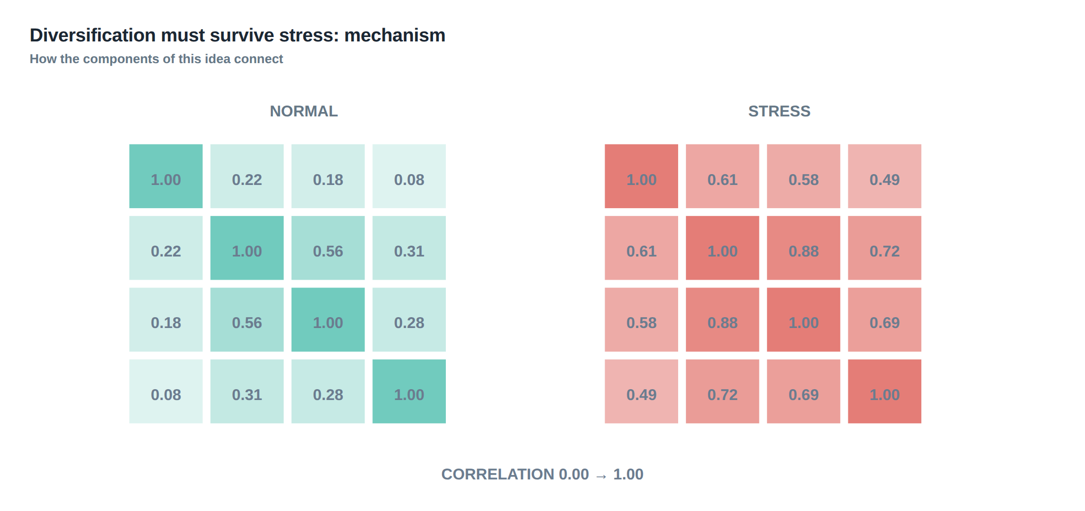
In calm markets the conditioning set \(\mathcal{F}_{t-1}\) contains modest volatility, ample liquidity and normal funding spreads. When a shock occurs – for instance a sudden 300‑basis‑point rise in overnight repo rates – the conditioning set expands to include high volatility, reduced depth and tighter margin constraints. The same two return series that once displayed a correlation of 0.12 can now exhibit 0.65 because both are forced to unwind positions into a thin order book.

A second mechanism is the interaction of factor shocks. Suppose a portfolio is exposed to a “short‑term funding” factor and a “liquidity‑drain” factor. In normal conditions the factor loadings are orthogonal, but a market stress that simultaneously raises funding costs and reduces market depth creates a linear combination of the two factors that is common to many strategies. The factor covariance matrix, therefore, becomes rank‑deficient, concentrating risk onto a single dominant eigenvector.

Third, the crowding effect amplifies the problem. When several desks hold similar statistical arbitrage signals, they all attempt to exit the same positions when a trigger is hit. The resulting order flow exceeds the market’s capacity to absorb it, causing spreads to widen and execution quality to deteriorate. The widening spreads feed back into the realised volatility of each strategy, inflating the correlation further.

Finally, margin calls act as a hard stop. If the portfolio’s net asset value falls below a pre‑set threshold, the clearing house issues a margin call that forces liquidation of the most liquid assets first. Because the liquidation is forced, the remaining positions are left with a higher proportion of illiquid exposure, which in turn raises the probability of further price impact. The cascade can be modelled as a stochastic process where the probability of a margin call at time \(t\) depends on the realised volatility and the liquidity‑adjusted concentration at \(t-1\).

A worked example with real numbers

Consider two systematic strategies run on the same desk:

Strategy Alpha trades a high‑frequency statistical‑arbitrage signal on US equity futures. Over the past 250 trading days it has delivered an average daily P&L of 0.08 % with a realised daily volatility of 1.2 %. The average daily correlation with the other strategy, measured over the same period, is 0.15.

Strategy Beta is a medium‑frequency macro‑driven futures spread that earns an average daily P&L of 0.06 % with a daily volatility of 0.9 %. Its average correlation with Alpha is 0.12.

On the surface the two strategies appear complementary: the combined portfolio volatility, using the historical correlation matrix, is

\[ \sigma_{p}=\sqrt{0.5\cdot1.2^{2}+0.5\cdot0.9^{2}+2\cdot0.5\cdot0.5\cdot0.15\cdot1.2\cdot0.9}\approx0.96\%, \]

and the expected daily return is 0.07 %, giving a Sharpe‑like ratio of roughly 0.73.

Now impose a stress scenario that mirrors a sudden funding squeeze observed in past market crises. The overnight repo rate spikes by 300 bps, the VIX doubles, and the average depth of the order book for the top ten futures contracts falls by 40 %. Under this environment we recompute the correlation matrix using a rolling 20‑day window that incorporates the stressed data. The correlation between Alpha and Beta jumps to 0.68 because both strategies now rely on the same thin pool of liquidity to fill orders.

Liquidity‑adjusted concentration is also recomputed. If the desk’s total capital allocated to the two strategies is £100 million, the liquidity‑adjusted exposure for Alpha rises from £30 million to £55 million, and for Beta from £20 million to £45 million, because each strategy now needs larger buffers to survive the wider spreads. The Herfindahl‑Hirschman Index (HHI) for liquidity‑adjusted exposure therefore moves from

\[ \text{HHI}_{\text{normal}}=\frac{30^{2}+20^{2}}{(30+20)^{2}}=0.34 \]

to

\[ \text{HHI}_{\text{stress}}=\frac{55^{2}+45^{2}}{(55+45)^{2}}=0.51, \]

indicating a marked increase in concentration.

When the stress persists for three days, the combined portfolio suffers a cumulative loss of 5 % (approximately 5.2 % for Alpha and 4.8 % for Beta), well beyond the daily VaR limit of 1 % that the desk had set based on the normal correlation matrix. The margin call threshold of 10 % drawdown is breached on day two, forcing an involuntary liquidation of the most liquid leg of Alpha’s position. The forced sell pressure widens the futures spread further, causing Beta’s P&L to deteriorate even more. The example demonstrates that low average correlation does not guarantee protection when the underlying liquidity and funding environment collapses.

Where it breaks in live markets

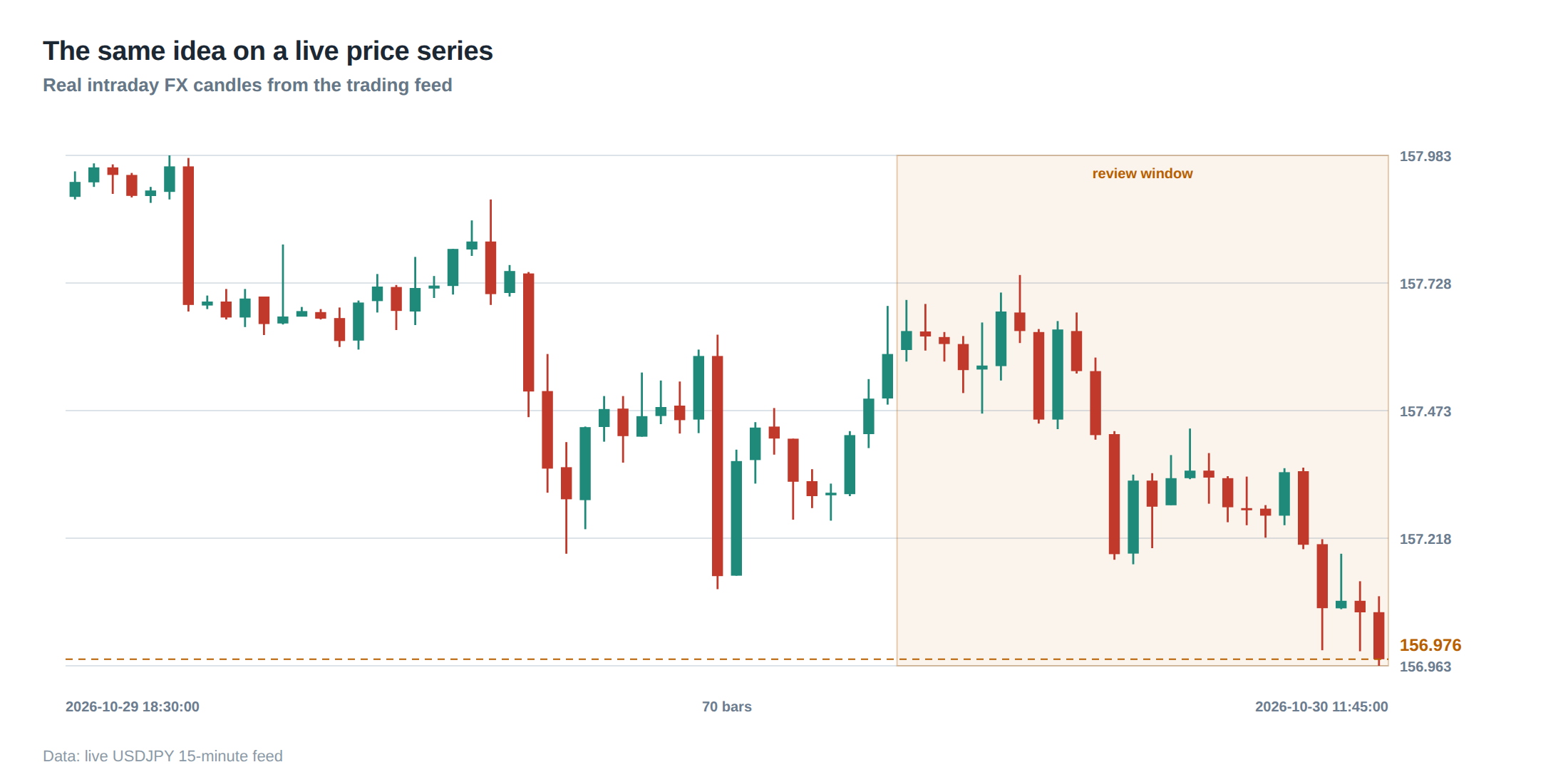
In practice the breakdown occurs at the intersection of three observable market signals: a rapid increase in realised volatility, a measurable widening of the bid‑ask spread on the instruments that constitute the majority of the desk’s exposure, and a spike in funding costs. The first signal is captured by a realised volatility index such as RVIX or a rolling standard deviation of 5‑minute returns. The second is measured by the average quoted spread across the top ten contracts, weighted by the desk’s notional exposure. The third is proxied by the overnight repo or Treasury‑funding spread.

When all three move in the same direction, the historical correlation matrix becomes obsolete. Empirically, during the 2020 COVID‑induced market shock, the average correlation among US equity futures rose from 0.13 to 0.71 within two trading sessions, while the average spread on the S&P 500 e‑mini doubled and the repo rate surged by 150 bps. The same pattern has been observed during the 2008 credit crisis and the 2022 European sovereign debt turmoil.

A further failure mode is the “crowded exit”. If ten desks are running similar high‑frequency arbitrage strategies, a single adverse news event can trigger simultaneous order flow in the same direction. The market’s depth is not a linear function of the number of participants; it collapses once the aggregate order size exceeds a threshold. The resulting price impact is non‑linear, and the realised correlation among the strategies spikes.

Margin calls compound the problem. The clearing house’s risk models typically use a 99 % VaR over a 10‑day horizon. When the realised volatility breaches that horizon, the margin call is issued, and the desk must liquidate positions regardless of the current market depth. The forced liquidation often occurs at the worst price in the order book, creating a feedback loop that further widens spreads and pushes other strategies into loss territory.

The operating path, stage by stage

The operating path that a prop desk should embed into its daily workflow can be described as a sequence of six stages.

Stage 1 – Baseline estimation: Compute the standard correlation matrix and factor loadings using a rolling window of 60‑day returns in a calm market regime. Store the eigen‑structure for later comparison.

Stage 2 – Stress‑signal monitoring: Continuously monitor three leading indicators – realised volatility, average spread, and funding cost – against pre‑defined thresholds (e.g., a 30 % increase in volatility over the 10‑day average, a 50 % spread widening, a 200 bps jump in repo).

Stage 3 – Dynamic matrix update: When any indicator breaches its threshold, recompute the correlation matrix using a shorter, more recent window (e.g., 10‑day) that captures the stressed dynamics. Record the new eigen‑values and compare the dominant eigenvector to the baseline.

Stage 4 – Liquidity‑adjusted concentration check: Recalculate the liquidity‑adjusted exposure for each strategy by dividing the notional exposure by the current average depth. Compute the HHI and compare it to a pre‑set limit (e.g., 0.45).

Stage 5 – Limit re‑calibration: If the stressed correlation exceeds a pre‑defined multiplier (e.g., 2 × the baseline average) or the HHI breaches its limit, automatically tighten position limits, reduce leverage, and raise the margin‑call buffer.

Stage 6 – Post‑event review: After the stress subsides, analyse the realised versus expected losses, update the stress‑scenario parameters, and feed the findings back into the baseline estimation.

Each stage is designed to be automated, with manual oversight only at the limit‑re‑calibration point. By structuring the workflow in this way, the desk ensures that diversification is re‑evaluated before the stress event erodes the very risk buffers it relied upon.

Controls that act before the damage

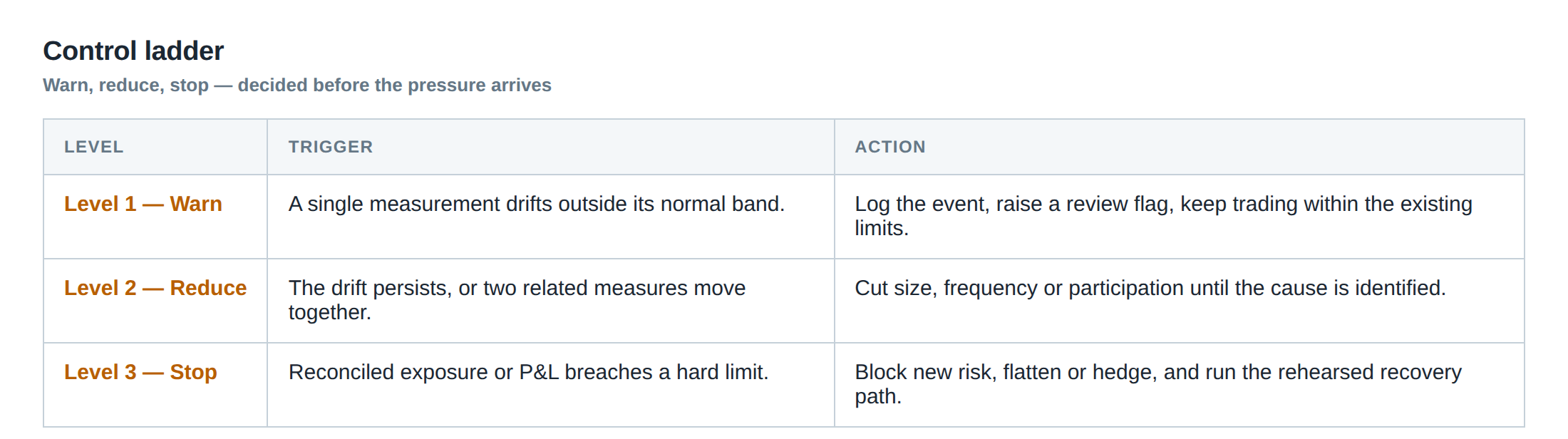
A layered control architecture – often visualised as a ladder – provides the final safeguard.

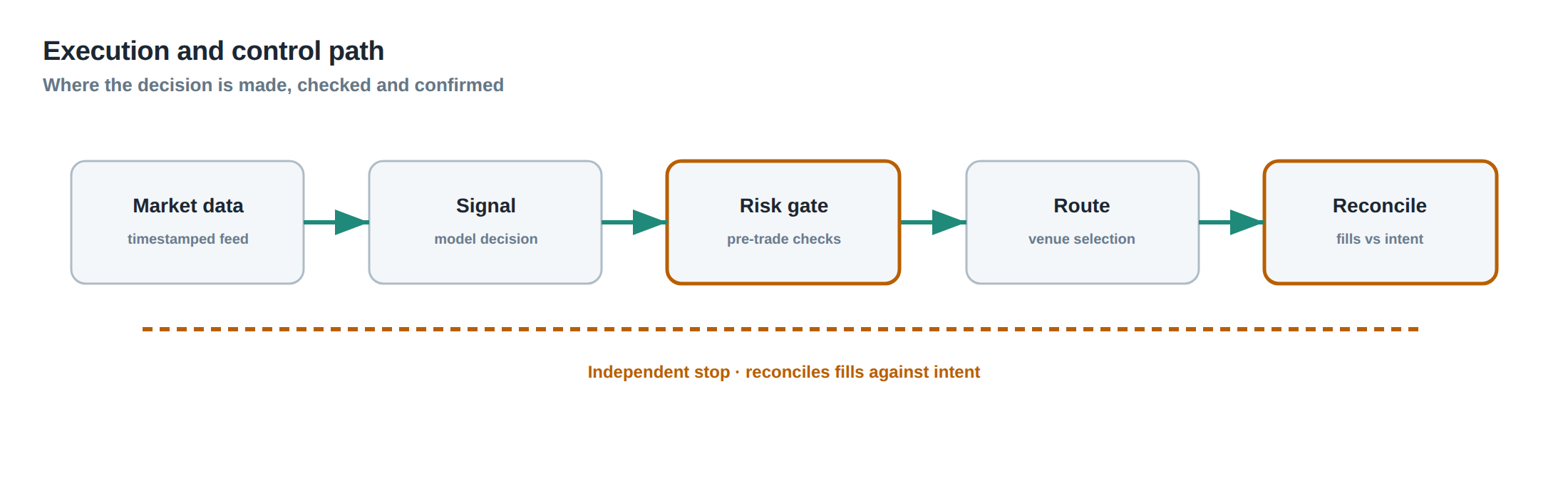
The first rung is pre‑trade validation. Before any order is sent, the system checks whether the current stressed correlation matrix would push the portfolio’s aggregate VaR above the daily limit. If so, the order is rejected or scaled down.

The second rung is intraday concentration monitoring. Real‑time dashboards display the liquidity‑adjusted HHI and flag any breach of the 0.45 threshold. When a breach occurs, the system automatically reduces the maximum allowable notional for the affected strategies.

The third rung is margin‑call buffer enforcement. Instead of waiting for the clearing house to issue a call, the desk maintains an internal buffer equal to 150 % of the official margin requirement. If the buffer falls below a set percentage of the portfolio equity, the system initiates a partial unwind of the most liquid positions.

The fourth rung is stress‑scenario back‑testing. Each night the desk runs a Monte‑Carlo simulation that injects simultaneous spread widening, volatility spikes, and funding shocks. The simulation generates a distribution of portfolio losses under stressed correlation matrices; the 99 % quantile is compared to the daily loss limit.

The final rung is governance escalation. If any of the above controls trigger more than three consecutive breaches, the desk’s risk committee must convene within one hour to decide whether to suspend trading on the affected strategies.

These controls act upstream of the loss event, ensuring that the portfolio never reaches a state where diversification has effectively disappeared.

How to measure whether it is working

Measurement hinges on two complementary metrics: stress‑adjusted VaR coverage and correlation‑drift detection lag.

Stress‑adjusted VaR coverage is the proportion of days on which the realised loss under stressed conditions stays within the VaR limit that was calculated using the stressed correlation matrix. A coverage of 95 % or higher indicates that the stress‑adjusted limits are appropriately calibrated.

Correlation‑drift detection lag measures the time elapsed between the first breach of a volatility or spread threshold and the moment the stressed correlation matrix is updated. The target lag is less than one trading hour; any longer lag suggests that the monitoring system is too sluggish to capture rapid market changes.

A third, more qualitative, indicator is the frequency of margin‑call buffer utilisation. If the buffer is invoked on more than 2 % of trading days, the underlying liquidity‑adjusted concentration limits may be too generous.

Regular reporting should include a heat map of the dominant eigenvalue of the correlation matrix over the past month, overlaid with the three stress indicators. A rising eigenvalue concurrent with widening spreads is a visual cue that diversification is eroding.

The portfolio view

From a portfolio‑management perspective, the key insight is that diversification is a dynamic, not static, attribute. The portfolio’s risk profile must be expressed as a function of market regime, not as a single point estimate.

When constructing a new strategy, the desk should first assess its liquidity footprint – the average depth required to execute its typical order size – and its funding sensitivity – the change in P&L for a one‑basis‑point move in overnight rates. These two dimensions become the primary axes of the stress‑scenario matrix.

During portfolio optimisation, the objective function should include a penalty term for liquidity‑adjusted concentration, alongside the traditional variance term. The penalty can be calibrated to the HHI threshold that triggers the second rung of the control ladder.

Finally, the portfolio view must incorporate exit‑contingency planning. For each strategy, the desk should pre‑define a “liquidity‑dry‑run” that simulates the impact of exiting 100 % of the position within a 30‑minute window under various spread scenarios. The resulting loss distribution feeds back into the daily limit‑setting process.

In sum, a portfolio that survives the worst market stress is one whose diversification has been continuously re‑validated against stressed correlation matrices, whose liquidity‑adjusted concentration is kept below a disciplined ceiling, and whose control ladder is capable of acting before the loss materialises.

Do you have a systematic way to detect when the correlation matrix you rely on has become obsolete?

About the research behind this lesson

Andrew Lo's lectures build risk analysis from return distributions and statistical measures, rather than treating one realised result as a complete description of risk.

Applied to this lesson: For a fast strategy, median latency or average fill quality is not enough. The review has to include tail delays, stale-order frequency and the loss distribution when cancellation or routing behaves abnormally.

Two live systems, one desk

PULSE-X — power-packed HFT: high-frequency momentum on XAUUSD and EURUSD. System details · Live account

NIC-X — ultra-low drawdown: displaced-print arbitrage for large capital. System details · Live account

Start now: leave your email and request a free trial — we will send the pricing, the connection route and the trial terms. Pricing

Join the market discussion: Telegram @squawklive

Source: Risk and Return

Educational content only. Trading leveraged products involves risk.