October 30, 2026

What this problem really is

When a desk imposes a per‑instrument limit it is often comforting to think that each trade lives in isolation. In reality the positions sit on a common set of risk drivers – a dollar‑wide risk‑on factor, a sector beta, a currency carry, a duration bucket, or a volatility regime. The aggregate exposure can be many times larger than the sum of the individual limits because the limits do not capture the correlation structure that binds the trades together. A modest long equity position in a US technology ETF, a short in a European high‑yield bond index, a futures contract on crude oil, a volatility swap, and a currency forward may all rise and fall together when the market switches from a risk‑off to a risk‑on stance. The resulting portfolio delta, beta, and volatility‑factor exposure can be equivalent to a single highly leveraged trade, even though each leg respects its own cap. The danger is not a single outlier move but the simultaneous alignment of several “small” bets on the same underlying driver.

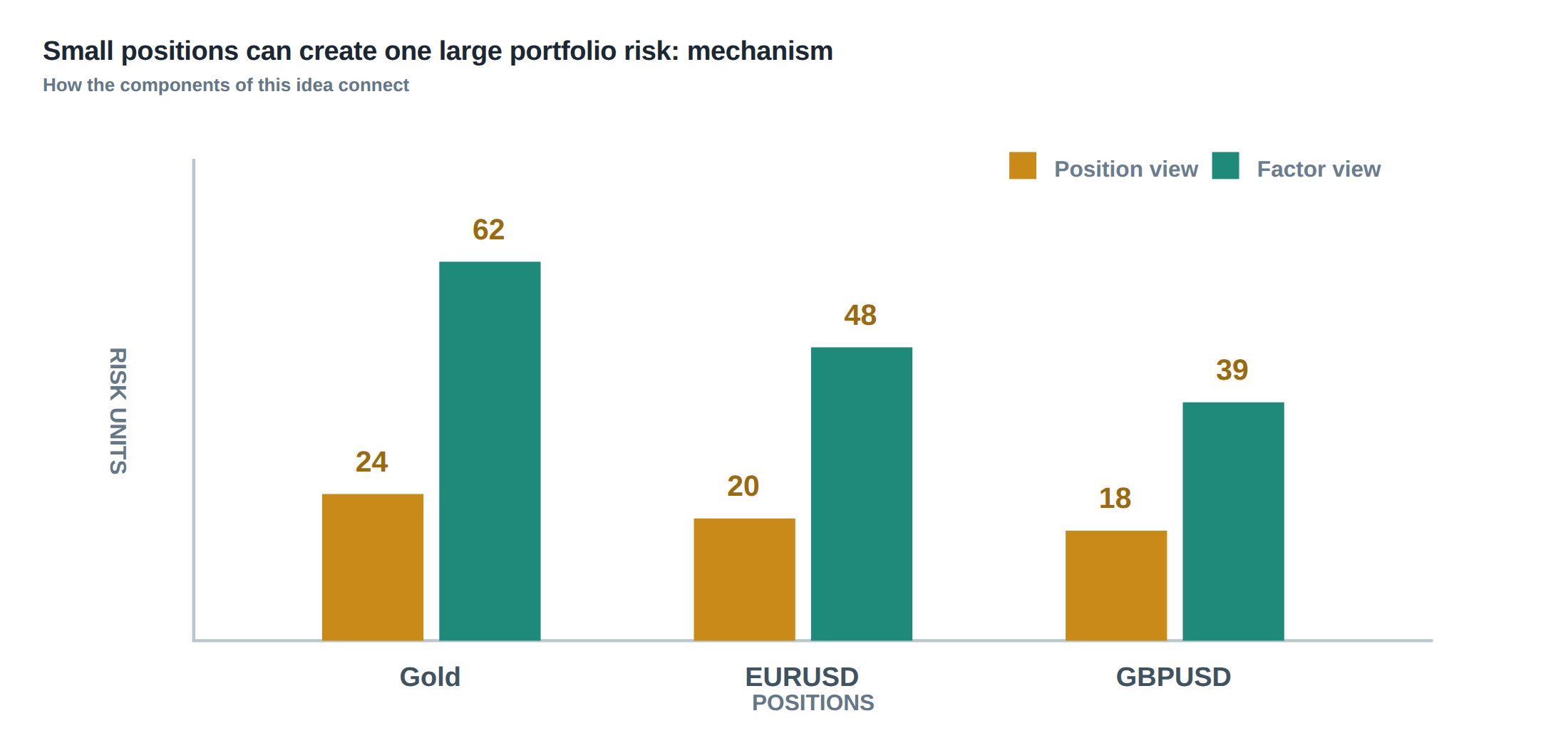
How the mechanism works, step by step

First, each strategy is decomposed into a set of risk factors – market beta, sector tilt, currency exposure, duration, and a set of liquidity‑related variables such as funding cost and market depth. The desk then measures the factor loadings of every instrument against a common factor library. Second, the factor loadings are summed across all active positions, producing an aggregate exposure vector. Third, the desk applies a stress matrix that inflates the correlations during periods of market stress; the matrix is calibrated on historical crisis windows rather than on calm‑period estimates. Fourth, the stressed aggregate exposure is compared against a set of concentration limits that are expressed in factor‑units rather than instrument‑units. Finally, if any factor limit is breached, the system automatically reduces or hedges the offending legs before the market can translate the latent exposure into realised loss.

A worked example with real numbers

Consider five positions that each sit comfortably under the desk’s per‑instrument limits: a 0.5 % long position in a US large‑cap equity index, a 0.4 % long position in a European equity index, a 0.6 % short position in a US high‑yield bond index, a 0.3 % long position in a crude‑oil futures contract, and a 0.2 % long position in a VIX futures contract. Individually each trade has a delta of less than 0.01 and a beta of less than 0.2 to the global market factor.

When the market enters a risk‑on episode the global dollar factor rises, European equities rally, high‑yield spreads tighten, oil prices climb, and implied volatility collapses. The factor loadings for each leg on the “risk‑on” driver are 0.8, 0.75, –0.7, 0.85 and –0.6 respectively. Summing the exposures gives a net risk‑on exposure of 0.8×0.5 % + 0.75×0.4 % – 0.7×0.6 % + 0.85×0.3 % – 0.6×0.2 % ≈ 0.71 % of the total capital. In a calm market the correlation matrix would suggest a modest net delta of 0.02, but under stress the same matrix inflates correlations by a factor of three, turning the net delta into roughly 0.06 – the equivalent of a 12‑times‑leverage on a single position.

If the desk’s aggregate risk‑on limit is set at 0.3 % of capital, the five “small” positions together breach the limit by more than double. The breach would be invisible if the desk only looked at gross exposure per instrument, but it becomes starkly apparent once the factor aggregation and stress amplification are applied.

Where it breaks in live markets

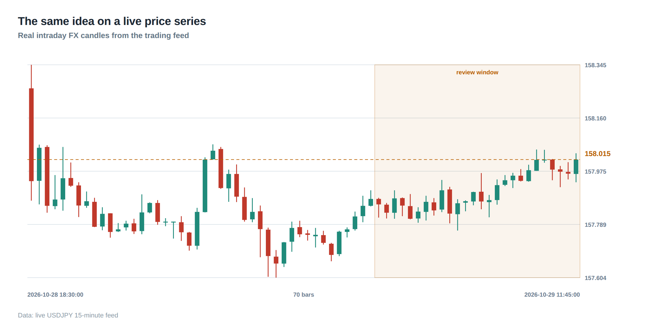
In live trading the breakdown usually occurs at the point where liquidity dries up and financing costs spike. When a market-wide shock hits, the shared funding source – for example, repo cash or short‑term commercial paper – can become scarce, causing the cost of carry on futures and forwards to rise sharply. The same shock also compresses order‑book depth, making the assumed linear price impact model invalid. Trades that were previously executed with sub‑tick slippage now suffer multi‑tick moves, and the realised volatility of the underlying jumps from 12 % to 35 % on an annualised basis.

Because the desk’s risk engine still relies on pre‑shock factor loadings, the realised portfolio beta can swing from 0.2 to 0.9 in a matter of minutes. The hidden concentration on the risk‑on factor therefore converts a series of modest losses into a single catastrophic drawdown. The failure mode is not a single instrument moving beyond its limit, but the simultaneous erosion of the assumptions that underpin all the limits – linear price impact, stable funding, and constant correlation.

The operating path, stage by stage

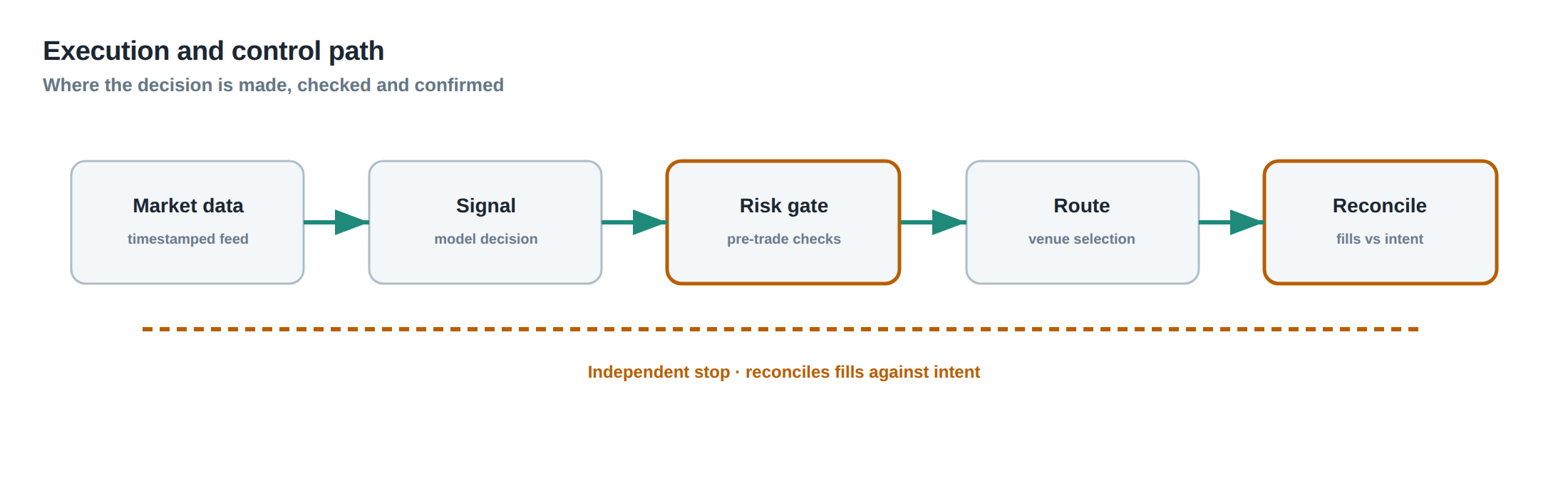
Stage one is data ingestion: market prices, funding rates, and order‑book snapshots are streamed into a central risk cache in real time. Stage two is factor decomposition, where each new order is projected onto the factor library using a pre‑computed loading matrix. Stage three aggregates the factor exposures across the entire book, updating the net vector every second. Stage four applies the stress matrix, which is itself a function of market‑wide stress indicators such as VIX, TED spread, and liquidity‑score thresholds. Stage five checks the stressed exposure against the factor‑level limits and raises alerts if any breach is imminent. Stage six either throttles the offending order flow or triggers a pre‑approved hedge, for example a short position in a market‑wide risk‑on ETF.

The flow is deliberately linear to avoid feedback loops that could amplify latency. Each stage has a hard deadline – for example, the aggregation step must complete within 150 ms – otherwise the system falls back to a conservative “kill‑switch” mode that stops new orders until the exposure can be reconciled.

Controls that act before the damage

The first line of defence is the pre‑trade factor limit. Before an order is sent to the market, the system calculates the marginal increase in each factor exposure and rejects the order if any would exceed the stressed limit. The second defence is a dynamic liquidity guard that monitors market depth and funding spreads; if depth falls below a configurable threshold the system raises a penalty factor that temporarily tightens the limits. The third defence is a scenario‑based stress test that runs every five minutes, injecting extreme moves in the common factors and checking whether the resulting exposure would breach capital‑at‑risk thresholds.

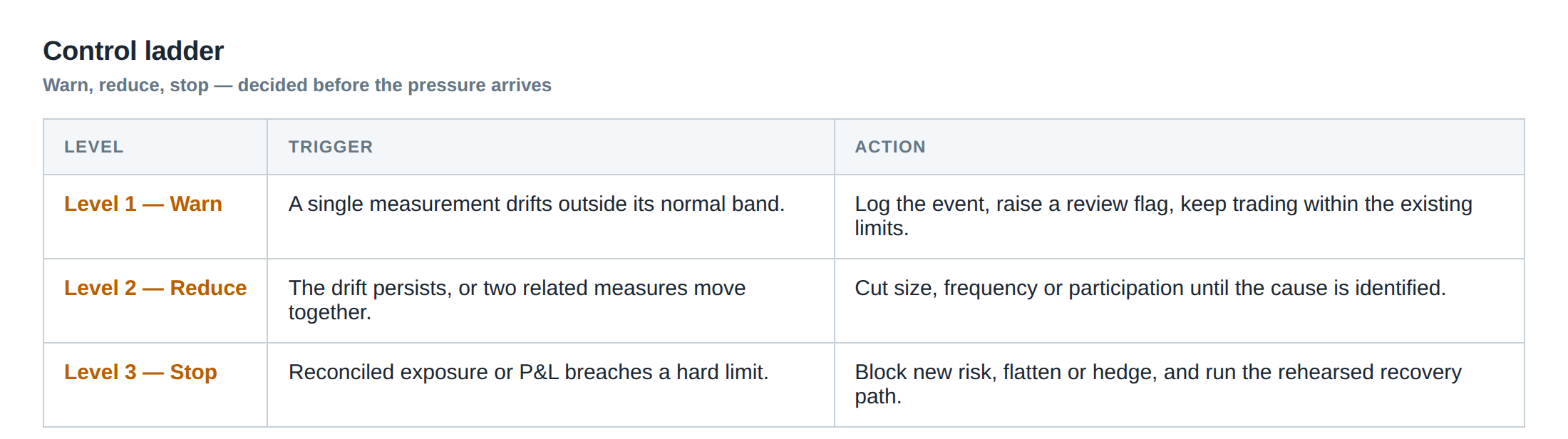
A fourth control is the “exposure ladder”, a visual representation that shows the current position of the portfolio on a multi‑dimensional risk surface. When the ladder approaches the top rung – the region where multiple factors are simultaneously near their limits – the system automatically reduces the size of new orders or forces a partial unwind of the most correlated legs. The ladder is updated in real time and feeds directly into the order‑routing engine, ensuring that the desk never accumulates hidden concentration.

How to measure whether it is working

The primary metric is the ratio of stressed aggregate exposure to the factor‑level limit, measured continuously. A value consistently below 0.7 indicates a comfortable buffer; a value that spends more than 5 % of trading time above 0.9 signals a control breach. Secondary metrics include the tail of the realised P&L distribution – the 99th percentile loss – and the frequency of “near‑miss” events where a single factor move of 1 % would have pushed the portfolio over its capital‑at‑risk ceiling.

Another useful gauge is the discrepancy between gross and net exposure under stress. If gross exposure is 1.2 % of capital but stressed net exposure inflates to 2.5 %, the system is exposing the desk to hidden leverage. Tracking the change in this discrepancy over time provides an early warning that correlations are tightening. Finally, the latency distribution of order acknowledgements under stress should be monitored; a shift of the 95th percentile from 30 ms to 120 ms often precedes a breakdown in the liquidity guard.

The portfolio view

From a portfolio perspective the aim is to treat the desk as a single, multi‑asset entity rather than a collection of independent desks. The aggregate delta, beta, currency, duration, and volatility‑factor exposures become the primary risk‑budget items, each with its own stressed ceiling. Gross exposure – the sum of absolute notionals – remains a useful sanity check, but the decisive figure is the stressed net exposure that incorporates correlation, liquidity, and funding stress.

By mapping each strategy to its shared liquidity and financing dependencies, the desk can see that a statistical arbitrage model, a macro‑funded carry trade, and a volatility‑selling program may all draw on the same repo market. When the repo market tightens, the combined funding pressure can force all three strategies to unwind simultaneously, creating a cascade that would be invisible if each strategy were examined in isolation.

Limiting concentration therefore requires a factor‑level approach: set caps on the total risk‑on exposure, on the aggregate currency‑hedge requirement, and on the net duration exposure across all fixed‑income legs. Scenario analysis should be run regularly, injecting extreme moves in each factor and observing the resulting portfolio loss. When the scenario loss exceeds a pre‑agreed percentage of capital, the desk must rebalance, either by reducing positions or by adding offsetting hedges that are uncorrelated with the stressed factor.

In practice, the portfolio view replaces the traditional per‑instrument limit with a dynamic, stress‑aware risk budget that recognises the hidden connections between seemingly small bets. The result is a more resilient book that can survive the same market shock that would otherwise turn five modest positions into a single, highly leveraged disaster.

Do you currently monitor your desk’s aggregate factor exposure under stressed correlation assumptions, or are you still relying on individual instrument limits alone?

About the research behind this lesson

Andrew Lo's lectures build risk analysis from return distributions and statistical measures, rather than treating one realised result as a complete description of risk.

Applied to this lesson: For a fast strategy, median latency or average fill quality is not enough. The review has to include tail delays, stale-order frequency and the loss distribution when cancellation or routing behaves abnormally.

Two live systems, one desk

PULSE-X — power-packed HFT: high-frequency momentum on XAUUSD and EURUSD. System details · Live account

NIC-X — ultra-low drawdown: displaced-print arbitrage for large capital. System details · Live account

Start now: leave your email and request a free trial — we will send the pricing, the connection route and the trial terms. Pricing

Join the market discussion: Telegram @squawklive

Source: Risk and Return

Educational content only. Trading leveraged products involves risk.