November 1, 2026

What this problem really is

The illusion of micro‑second precision is a frequent source of spurious alpha in high‑frequency trading (HFT). When the timestamps attached to market data, order submissions and execution reports are not generated from a single, synchronised clock, the apparent sequence of events can be inverted. A back‑test that relies on the recorded times will then attribute causality to a trade that, in reality, arrived after the price move it is claimed to have anticipated. The resulting “alpha” is a statistical artefact, not a reproducible edge.

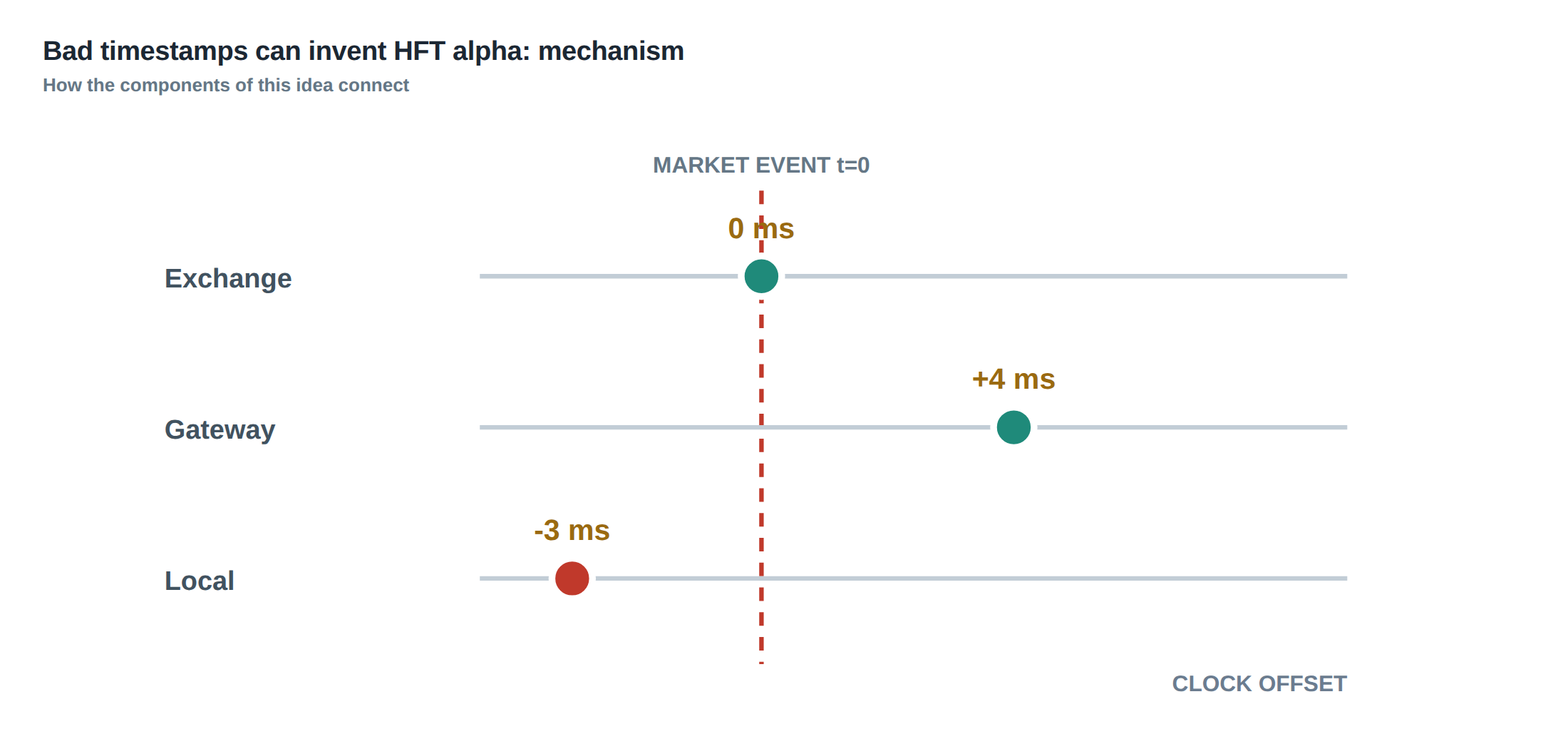
The root cause is the heterogeneous nature of the data path. Exchanges publish quote and trade feeds from separate servers, each with its own timing discipline. Gateway appliances add another layer of timestamps, often derived from the operating system clock, which may be offset by several microseconds from the exchange’s reference. Finally, the local receive timestamp recorded by the strategy engine can be delayed by kernel scheduling, network driver queues or NIC timestamping inaccuracies. When these three timestamps are treated as interchangeable, the chronology of market events becomes unreliable.

For a prop‑trading desk that trades on sub‑millisecond windows, the distinction between “when the market moved” and “when the system recorded the move” is decisive. An apparent lead of even a few microseconds can inflate Sharpe ratios, hide latency outliers, and misguide risk models. The problem is therefore not merely academic; it can cause the deployment of strategies that appear profitable in simulation but crumble when confronted with the true ordering of market information.

How the mechanism works, step by step

First, the exchange timestamps each quote update and each trade execution with its own clock, typically synchronised to a GPS‑derived time source. These timestamps travel embedded in the data packets, but they are not the only time reference that reaches the trader. The gateway that aggregates the feeds adds a receipt timestamp based on the host’s kernel clock, which may be subject to NTP adjustments or drift relative to the exchange’s clock.

Second, the trader’s order management system (OMS) creates an order‑submission timestamp at the moment the API call is issued. This timestamp is recorded before the order traverses the network to the exchange’s matching engine. The exchange then timestamps the order acceptance, the subsequent fill, and any cancellation, each using its own clock. The OMS finally records a local receipt timestamp when the acknowledgement arrives.

Third, the strategy logic consumes the data stream using the timestamps it receives. If the logic assumes that the exchange‑provided quote timestamp is the definitive moment the market changed, it will ignore the fact that the trade timestamp may have been generated later, even though the trade packet arrived earlier on the network. The mismatch can cause the strategy to “see” a price move before it actually occurred, creating the illusion of predictive power.

The final step is the back‑test, which typically orders events by the local receipt timestamps. Without explicit correction for clock offset and drift, the back‑test will preserve the inverted ordering, leading to a systematic bias that favours strategies that appear to act on information before it is truly available.

A worked example with real numbers

Consider a simple mean‑reversion scalp that triggers when the mid‑price drops by 0.5 bps within 200 µs. The exchange publishes a quote update at 09:30:00.123456 UTC, timestamped 09:30:00.123456. Ten microseconds later, at 09:30:00.123466, a trade for 10 k contracts executes at a price 0.6 bps lower, and the exchange timestamps this trade as 09:30:00.123466.

The gateway receives the trade packet first, because the trade feed uses a lower‑latency multicast channel, and records a local receipt timestamp of 09:30:00.123470. The quote packet arrives 8 µs later on a higher‑latency channel, and the gateway stamps it as 09:30:00.123478. The OMS, unaware of the offset, orders the events by these local timestamps: trade first, then quote. The strategy therefore believes the price moved before the quote reflected it, and generates a sell order at 09:30:00.123480, which is recorded as a profitable fill.

In reality, the quote change preceded the trade by 10 µs; the apparent lead is an artefact of the mismatched feed latencies and unsynchronised timestamps. If the back‑test uses the exchange timestamps directly, the trade would be placed after the quote, and the strategy would miss the entry. The spurious profit in the back‑test is thus entirely due to the bad timestamp alignment.

If we introduce a measured clock offset of +4 µs between the exchange and the gateway, and a drift of –0.2 µs per minute, we can correct the timestamps: the trade’s corrected time becomes 09:30:00.123462, and the quote’s corrected time 09:30:00.123474. The corrected ordering now matches the true market sequence, and the strategy no longer generates the false signal. This numerical illustration demonstrates how a few microseconds of mis‑alignment can fabricate alpha that vanishes once proper timing discipline is applied.

Where it breaks in live markets

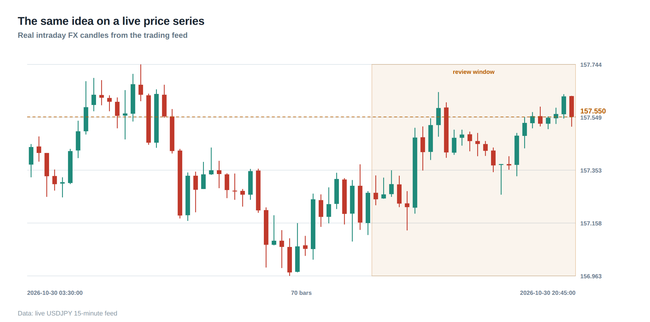
In production, the problem is amplified by several practical realities. Network congestion can cause packets to be delayed by tens of microseconds, and the variability of those delays is not captured by a single average latency figure. Moreover, exchange‑wide clock adjustments, such as leap‑second handling or GPS lock loss, introduce sudden jumps in the reference time that propagate through the feed without immediate detection.

Another failure mode is the handling of correction messages. Exchanges occasionally resend a quote with a revised timestamp to rectify an earlier mis‑timestamp. If the strategy discards the original message without preserving its sequence number, it may double‑count a price level or miss a rapid reversal. Duplicate events, arising from network retransmissions, can also corrupt the event stream if not filtered based on unique identifiers.

Finally, the latency tail – the worst‑case delay observed in a given interval – often exceeds the median by an order of magnitude. A strategy that only monitors median latency will be blind to occasional outliers that reorder events. When a tail delay pushes a quote receipt beyond a trade receipt, the strategy may act on stale information, leading to execution at unfavourable prices and a rapid erosion of the apparent edge.

The operating path, stage by stage

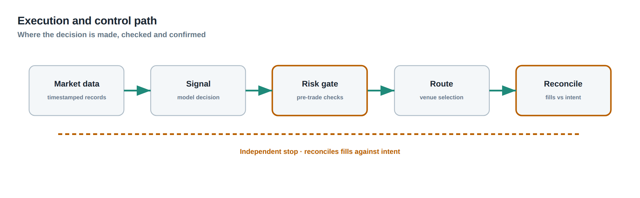
The first stage is the exchange feed ingestion. Here the system should store the raw exchange timestamp, the gateway receipt timestamp and the local receive timestamp as three distinct fields attached to each event. By preserving the three‑point time vector, later analysis can reconstruct the true ordering and quantify the offset at any moment.

The second stage is the order‑routing layer. Each outbound order must be tagged with a locally generated submission timestamp and a sequence identifier. The acknowledgement from the exchange, bearing its own timestamp, is logged alongside the local receipt timestamp. This dual‑recording enables detection of cases where the order was accepted after a market move that the strategy thought it preceded.

The third stage is the event‑processing engine. It must maintain the original sequence numbers supplied by the exchange and apply a deterministic rule for handling out‑of‑order arrivals: for example, buffering events for a short, configurable window (e.g., 20 µs) and then re‑ordering them according to the exchange timestamps before they enter the strategy logic.

The fourth stage is the risk‑monitoring subsystem. It continuously computes the offset between the exchange and gateway clocks, as well as the drift over longer periods, and raises alerts when the offset exceeds a pre‑defined threshold (e.g., 5 µs). It also tracks the frequency of duplicate or corrected messages, feeding that information back to the ingestion stage to adjust buffering parameters.

By structuring the pipeline into these clearly defined stages, the desk can isolate the source of timing anomalies and apply corrective measures without disrupting the entire system.

Controls that act before the damage

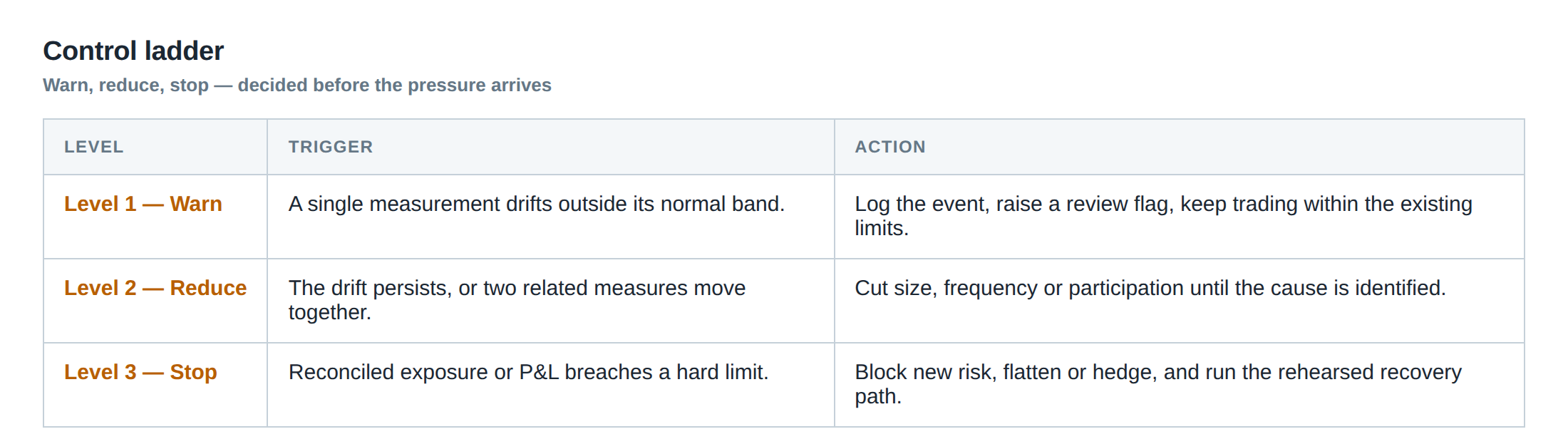
At the hardware level, the use of NICs that support hardware timestamping reduces the variability introduced by the operating system. Deploying a Precision Time Protocol (PTP) grandmaster on the same LAN as the gateway ensures that the gateway clock stays within sub‑microsecond synchronisation of the exchange’s reference.

Software controls include a timestamp‑validation module that checks each incoming packet for monotonicity of the exchange timestamps. When a non‑monotonic sequence is detected, the module flags the event and forces the processor to pause the strategy for a brief back‑pressure period, allowing the buffer to catch up and re‑order the events correctly.

A further safeguard is the implementation of a “latency ladder” that records the distribution of the three‑point time differences for each event class (quotes, trades, acknowledgements). The ladder visualises the tail behaviour and triggers an automatic throttling of order flow if the 99.9th percentile exceeds a safety limit. This pre‑emptive control prevents the strategy from acting on stale data during periods of network stress.

Finally, operational procedures mandate daily calibration of the clock offset using a known reference feed, such as a time‑synchronised market data replay. The calibration results are stored in a configuration file that the ingestion stage reads at start‑up, ensuring that the system begins each trading day with an accurate baseline offset.

How to measure whether it is working

The primary metric is the post‑trade “information latency”: the elapsed time between the exchange timestamp of the market event that justified the trade and the local receipt timestamp of the trade acknowledgement. By aggregating this metric over a rolling window, the desk can observe whether the median and tail latencies remain within the target envelope.

A secondary measure is the “re‑ordering rate”, defined as the proportion of events that required buffer‑based re‑sequencing because their arrival order differed from the exchange timestamp order. A low re‑ordering rate (below 0.1 %) indicates that the clock alignment and network paths are stable.

The third indicator is the frequency of correction and duplicate messages that survive to the strategy layer. These should be logged and compared against the expected rate published by the exchange; a sudden increase signals a possible timing drift or feed‑integrity issue.

Finally, a back‑test that re‑runs historical data with the corrected timestamps should produce performance metrics that are statistically indistinguishable from the live results. Any divergence points to residual timing bias that must be investigated. By monitoring these quantitative signals, the desk can certify that the timestamp discipline is effective.

The portfolio view

When the timing controls are robust, the portfolio’s risk profile reflects the true execution quality rather than an artefact of mis‑ordered data. The tail of the latency distribution becomes a genuine component of the risk model, allowing the desk to allocate capital based on realistic worst‑case scenarios.

Conversely, if bad timestamps persist, the portfolio will exhibit unexplained spikes in realised P&L that disappear when the strategy is run on a correctly ordered data set. Such spikes often correlate with periods of network congestion or exchange clock adjustments, and they inflate the apparent Sharpe ratio while masking hidden exposure to stale‑order risk.

Integrating timestamp validation into the portfolio analytics pipeline ensures that performance attribution is grounded in actual market dynamics. It also enables more accurate stress testing, as the simulated latency tails now match the observed tails, preventing the underestimation of drawdown risk. In a competitive prop‑trading environment, this level of fidelity is essential for sustaining an edge that is not merely a statistical illusion.

Do you have a process in place to verify that the timestamps you rely on truly reflect the market’s chronology, and can you quantify the impact of any mis‑alignment on your strategy’s performance?

About the research behind this lesson

Andrew Lo's lectures build risk analysis from return distributions and statistical measures, rather than treating one realised result as a complete description of risk.

Applied to this lesson: For a fast strategy, median latency or average fill quality is not enough. The review has to include tail delays, stale-order frequency and the loss distribution when cancellation or routing behaves abnormally.

Two live systems, one desk

PULSE-X — power-packed HFT: high-frequency momentum on XAUUSD and EURUSD. System details · Live account

NIC-X — ultra-low drawdown: displaced-print arbitrage for large capital. System details · Live account

Start now: leave your email and request a free trial — we will send the pricing, the connection route and the trial terms. Pricing

Join the market discussion: Telegram @squawklive

Source: Risk and Return

Educational content only. Trading leveraged products involves risk.