November 1, 2026

What this problem really is

When a back‑test finishes, the analyst is left with a tidy distribution of returns, a Sharpe ratio and a handful of risk metrics. Those numbers are derived from a closed‑loop where every order is assumed to be accepted, filled at the quoted price and cleared instantly. In reality the live stack is a chain of asynchronous components – market data feed, order router, risk engine, execution venue and settlement system – each of which can introduce delays, rejections or outright failures. The moment the strategy moves from a simulated environment to a production broker, the “missing” failure modes begin to surface. The back‑test therefore represents a best‑case scenario, not a complete description of the risk the strategy will face once it is deployed.

Historical returns ignore three broad categories of production risk. First, timing risk: latency, jitter and out‑of‑order messages can turn a profitable slice of the order book into a stale quote. Second, execution risk: partial fills, order rejects, and venue‑specific throttling can erode expected slippage and turn a theoretical fill into a half‑filled position. Third, infrastructure risk: disconnects, data gaps and stale market data can cause the algorithm to act on information that no longer reflects the market. The cumulative effect of these factors can transform a strategy that appears robust in back‑test to one that is consistently untradeable in live markets.

How the mechanism works, step by step

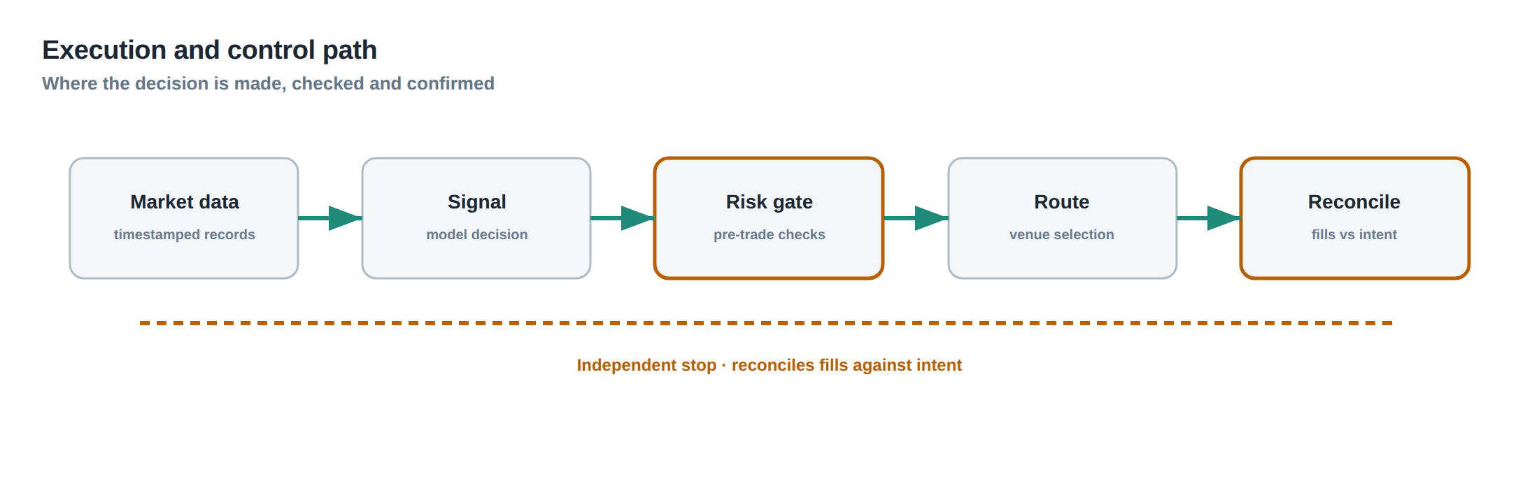
The live pipeline begins with a market‑data subscription. A feed handler timestamps each tick, normalises the format and pushes the message into a shared queue. The strategy thread consumes the queue, computes a signal and creates an order object. That object is handed to a risk manager, which checks position limits, margin and compliance rules before forwarding the request to an order router. The router selects a venue, attaches a unique client order identifier and transmits the message over a TCP socket.

On the exchange side, the order enters an order‑book matching engine. If the venue’s internal latency exceeds the strategy’s expectation, the order may be queued behind a burst of higher‑priority traffic. The exchange can reject the order outright (e.g. due to a malformed field) or acknowledge it with a delayed execution report. The execution report is routed back through the same network path, where it may be delayed, reordered or dropped. The strategy must therefore reconcile its internal state with a possibly stale view of the market, and decide whether to cancel, replace or let the order sit.

If the order is filled, a fill message arrives, again subject to latency and possible partial execution. The algorithm updates its position, calculates realised P&L, and may immediately generate a hedge or a stop‑loss order. Each of these subsequent messages is exposed to the same latency and reliability constraints. The end‑to‑end latency distribution – from signal generation to fill confirmation – is therefore a convolution of many stochastic processes, not a single deterministic number.

A worked example with real numbers

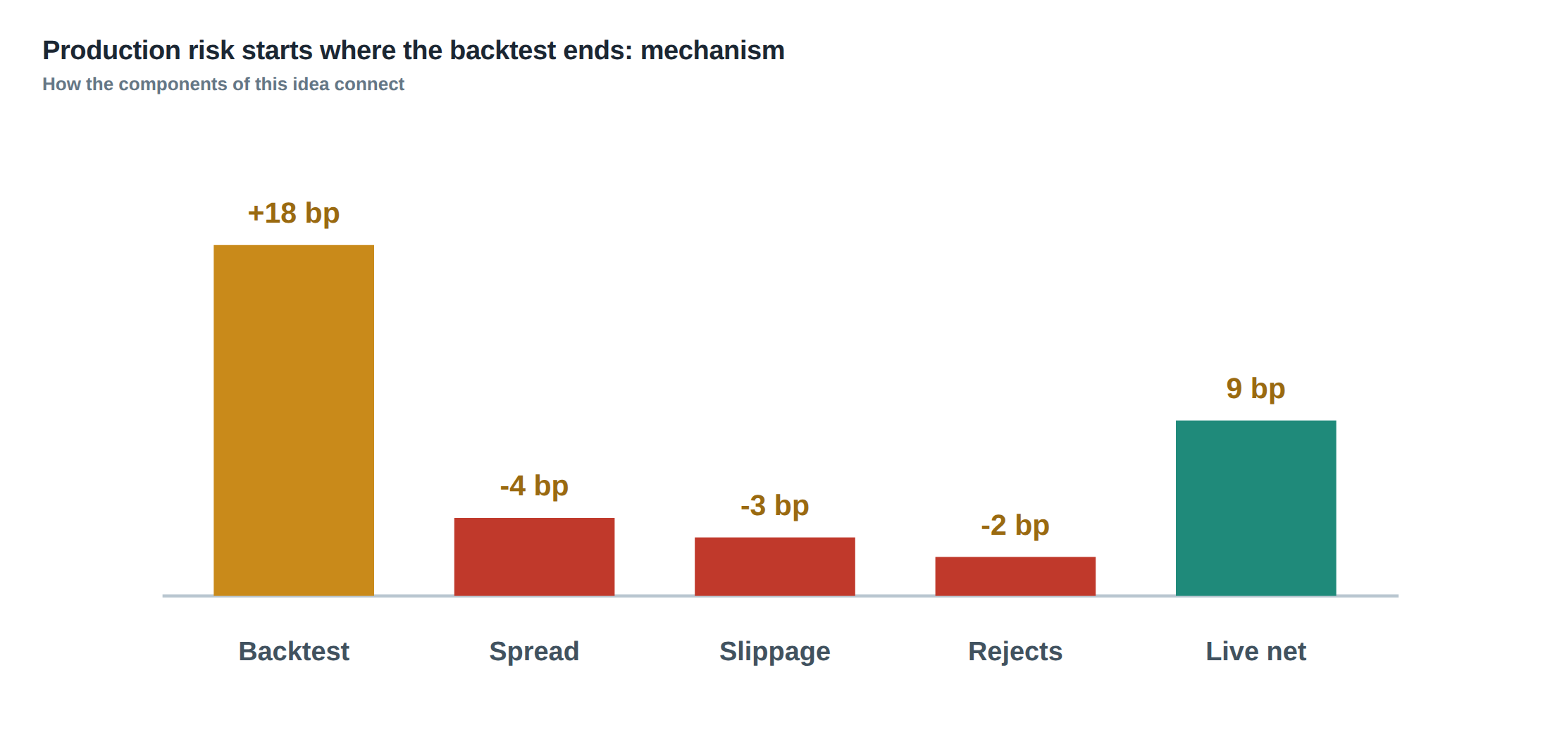
Consider a mean‑reversion signal that looks for a 0.3 % deviation in a liquid futures contract and places a market‑on‑close (MOC) order to capture the reversion. In back‑test the signal produces an average gross return of 0.45 % per trade, with a median fill latency of 12 ms and a standard deviation of 4 ms. Transaction costs are modelled as a flat 0.04 % commission plus a 0.02 % slippage, leaving a net expected profit of 0.39 % per trade.

In live deployment the same signal fires 1 000 times over a week. The average round‑trip latency measured from timestamped signal to fill confirmation is 18 ms, but the 99th‑percentile latency spikes to 62 ms because of a brief congestion episode on the exchange gateway. During those spikes the MOC order arrives after the market close, and the exchange returns a “order rejected – market closed” message. The algorithm, unaware of the rejection until 70 ms later, proceeds to send a replacement limit order at the stale price, which is subsequently filled at a price 0.12 % worse than the original target.

The net effect is a reduction of realised profit per trade from 0.39 % to 0.21 %. Moreover, 84 of the 1 000 trades are either partially filled (average fill ratio 62 %) or fully rejected, turning a theoretically profitable signal into a loss‑making operation for that week. The back‑test never captured the tail of the latency distribution, nor the interaction between overlapping replacement orders and the exchange’s order‑book state.

Where it breaks in live markets

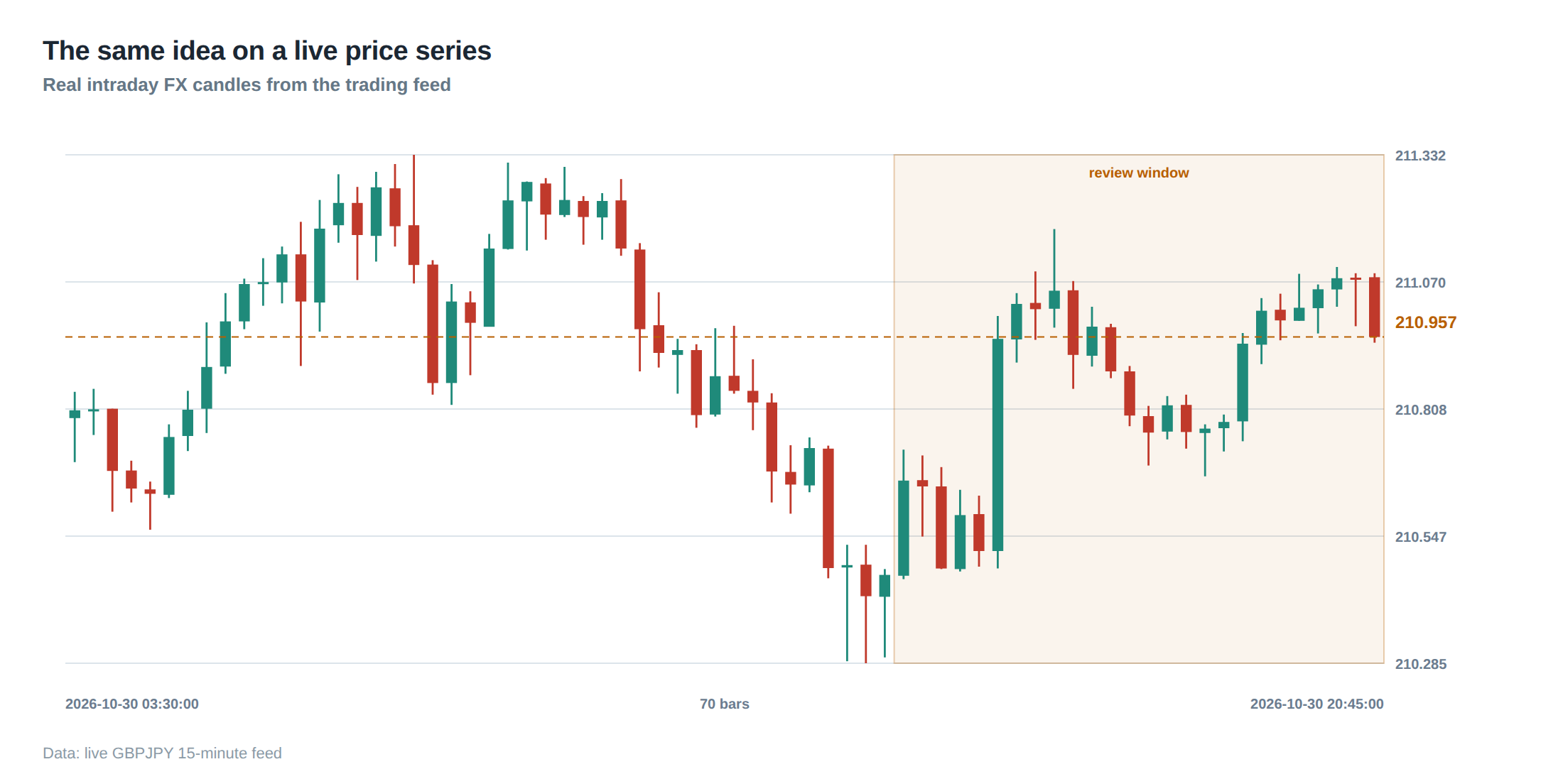
The first point of failure is often the data feed. If a broker’s snapshot is delayed by even a few milliseconds, the algorithm may calculate a signal based on a price that has already moved beyond the profitable region. Stale data can also arise from packet loss; a missing tick can cause the algorithm to mis‑interpret a price swing as a trend reversal, prompting an ill‑timed entry.

A second failure mode is order rejection. Exchanges enforce a variety of constraints – minimum order size, price increments, and risk limits – that may differ from the assumptions baked into the back‑test. A sudden change in venue‑level throttling can cause the router to exceed the allowed message rate, resulting in a “rate limit exceeded” reject. The strategy may then flood the gateway with replacement orders, each of which inherits the same latency penalty, creating a feedback loop that amplifies the initial delay.

Third, partial fills introduce a hidden exposure. The back‑test assumes a full execution at the quoted price, but in a thin market a 100 % fill may be impossible. The remaining unfilled quantity sits exposed to adverse price movement, and the algorithm’s risk model – calibrated on full fills – underestimates the true exposure.

Finally, infrastructure outages – network partition, broker API downtime, or hardware failure – can freeze the entire order flow. Even a brief disconnect can cause the strategy to miss the execution window entirely, turning a high‑probability trade into a missed opportunity.

The operating path, stage by stage

The production stack can be visualised as a linear chain of stages, each with its own latency envelope and failure probability. Stage 1 is market‑data ingestion, where timestamp accuracy and message ordering are verified. Stage 2 is signal generation, where the algorithm consumes the normalised data and produces an order intent. Stage 3 is risk validation, which checks capital, position limits and compliance flags. Stage 4 is routing, where the order is encoded, signed and dispatched to the chosen venue. Stage 5 is venue acceptance, where the exchange either acknowledges, rejects or queues the order. Stage 6 is execution, where a fill report is generated and returned. Stage 7 is post‑trade processing, where P&L, inventory and performance metrics are updated.

Each stage contributes additively to the overall latency distribution, but multiplicatively to the probability of an abnormal outcome. For example, a 0.5 % chance of a data‑feed gap combined with a 0.2 % chance of a router timeout yields a joint probability of roughly 0.001 % for a “gap‑plus‑timeout” scenario. Although rare, such tail events dominate the loss distribution for high‑frequency strategies where the profit per trade is measured in basis points.

Controls that act before the damage

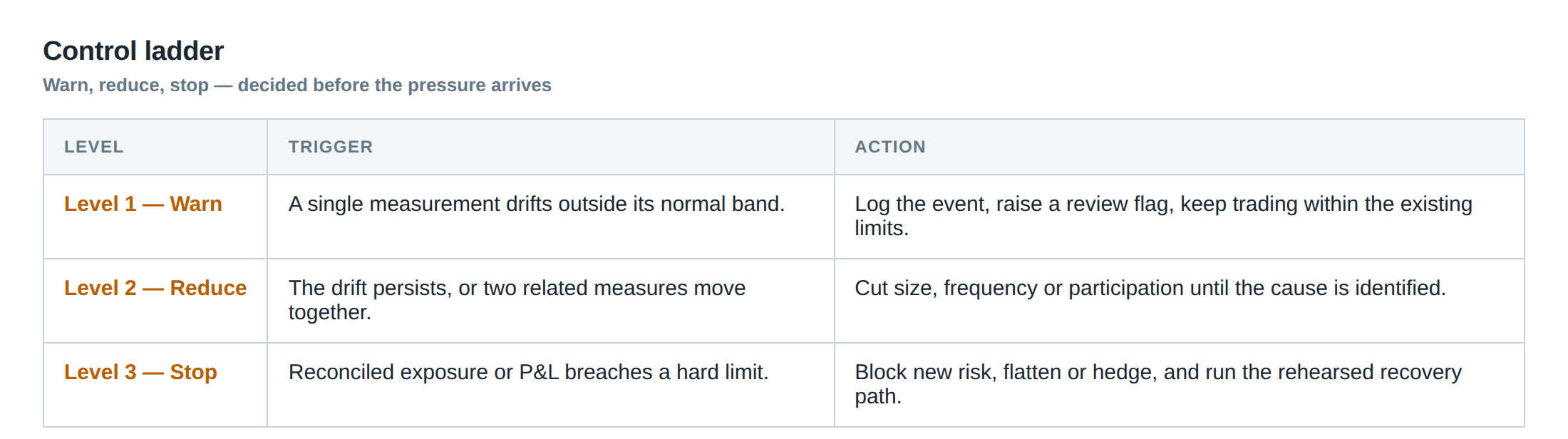
A robust production system embeds safeguards at every stage of the chain. At the data‑feed layer, sequence numbers and checksum validation reject out‑of‑order or corrupted packets before they reach the strategy. Time‑synchronisation protocols such as PTP (Precision Time Protocol) ensure that timestamps across the stack are aligned to within a microsecond, reducing the risk of stale‑order generation.

Risk validation is hardened by dynamic limits that adapt to recent latency spikes; if the median round‑trip latency exceeds a pre‑set threshold, the system automatically reduces order size or switches to a more forgiving venue. The router incorporates a back‑off algorithm that throttles order submissions when the exchange returns rate‑limit rejections, preventing a cascade of duplicate orders.

On the execution side, the algorithm monitors fill quality in real time. If the fill ratio falls below a configurable floor (for instance 70 % of the requested quantity), the strategy aborts the remaining exposure and issues a market‑on‑close unwind order. Partial‑fill handling is baked into the position manager, which re‑calculates the risk‑adjusted P&L after each incremental fill.

Finally, a shadow‑trading environment mirrors the live stack but with a zero‑capital allocation. Orders are sent through the same gateway, the same risk checks, and the same data feed, yet the execution reports are discarded. The shadow trader records latency, reject rates and fill ratios, providing a live benchmark against which the research‑phase metrics can be compared.

How to measure whether it is working

Measurement begins with a granular latency histogram for each stage of the pipeline. The median, mean and, crucially, the 95th and 99th percentiles must be tracked daily. A widening tail indicates emerging congestion or a degradation in network quality.

Reject and partial‑fill rates are recorded as percentages of total order flow, and are broken down by venue, order type and time‑of‑day. The distribution of fill ratios should be compared to the back‑test assumption of 100 % fills; any systematic shortfall is a signal that the execution model needs recalibration.

Stale‑order frequency is measured by comparing the timestamp of the market data used to generate a signal with the timestamp of the order acknowledgement. If the gap exceeds the acceptable latency window (for example 30 ms for a sub‑millisecond strategy), the order is flagged as stale. The proportion of stale orders over a rolling window provides a direct indicator of the effectiveness of the data‑feed validation layer.

The shadow‑trader’s performance metrics – realised P&L, win‑rate, average slippage – are plotted alongside the live strategy’s metrics. Divergence beyond a pre‑defined tolerance (e.g. 5 % difference in average slippage) triggers a review of the routing logic or a temporary reduction in capital allocation.

The portfolio view

From a portfolio perspective, production risk manifests as an unexpected drag on the risk‑adjusted return. The realised Sharpe ratio will typically be lower than the back‑tested figure, not because the underlying alpha has vanished, but because the cost of latency, rejects and partial fills adds a hidden loss component.

When aggregating multiple strategies, the correlation of their production‑risk profiles becomes critical. If several high‑frequency signals share the same data feed or router, a single latency spike can simultaneously impair all of them, creating a concentration of tail risk that is invisible in the individual back‑tests. Portfolio‑level stress tests should therefore inject synthetic latency spikes and reject bursts into the live‑order simulator, measuring the joint impact on capital utilisation and drawdown.

A disciplined allocation framework reserves a buffer of capital – often termed “production capital” – that can absorb the excess losses attributable to production risk. The size of this buffer is calibrated by the historical variance of the loss‑distribution tail, not by the mean return. By monitoring the buffer’s utilisation over time, the desk can decide when to scale a strategy up, keep it at current levels, or pull it back entirely.

In summary, the gap between back‑tested returns and live performance is largely a product of unmodelled production risk. By replaying realistic message order and latency, simulating rejects, partial fills, disconnects and stale data, and by embedding shadow‑trade monitoring, a prop‑trading desk can close that gap and protect the portfolio from hidden loss sources.

What steps will you take today to audit the production‑risk assumptions of your own strategies?

About the research behind this lesson

Andrew Lo's lectures build risk analysis from return distributions and statistical measures, rather than treating one realised result as a complete description of risk.

Applied to this lesson: For a fast strategy, median latency or average fill quality is not enough. The review has to include tail delays, stale-order frequency and the loss distribution when cancellation or routing behaves abnormally.

Two live systems, one desk

PULSE-X — power-packed HFT: high-frequency momentum on XAUUSD and EURUSD. System details · Live account

NIC-X — ultra-low drawdown: displaced-print arbitrage for large capital. System details · Live account

Start now: leave your email and request a free trial — we will send the pricing, the connection route and the trial terms. Pricing

Join the market discussion: Telegram @squawklive

Source: Risk and Return

Educational content only. Trading leveraged products involves risk.