November 7, 2026

What this problem really is

The temptation on a prop desk is to treat each trade as an isolated experiment, imposing a hard notional cap or a simple delta limit on the individual position. In practice those caps ignore the fact that the five modest longs in the example are all exposed to the same underlying driver – a dollar‑strength, risk‑on bias that surfaces whenever market participants shift from safe‑haven assets to equity‑risk assets. When that bias spikes, the five positions move together, multiplying the effective exposure far beyond the sum of their stand‑alone limits. The result is a hidden lever that can wipe out a quarter of the capital pool in a single adverse move.

The root cause is the failure of “individual limits” to capture common‑factor exposure. A portfolio of futures, ETFs, and cash‑secured forwards may each sit comfortably under a 2 % delta ceiling, yet their aggregate beta to the US dollar, their shared funding cost, and their joint volatility sensitivity can sum to a net exposure equivalent to a 20 % leveraged trade. The risk is not visible in a static snapshot; it emerges only when the factor that binds the trades is stressed.

Academic work on risk measurement shows that a single realised return does not describe the full distribution of outcomes. By focusing on the tail of the distribution – the rare but severe co‑movements – a desk can see that the apparent safety of small positions is illusory. The same logic that drives a median latency analysis for a high‑frequency strategy applies to portfolio construction: the median fill quality is insufficient, the tail of execution delays and stale‑order incidents must be incorporated into the loss distribution.

How the mechanism works, step by step

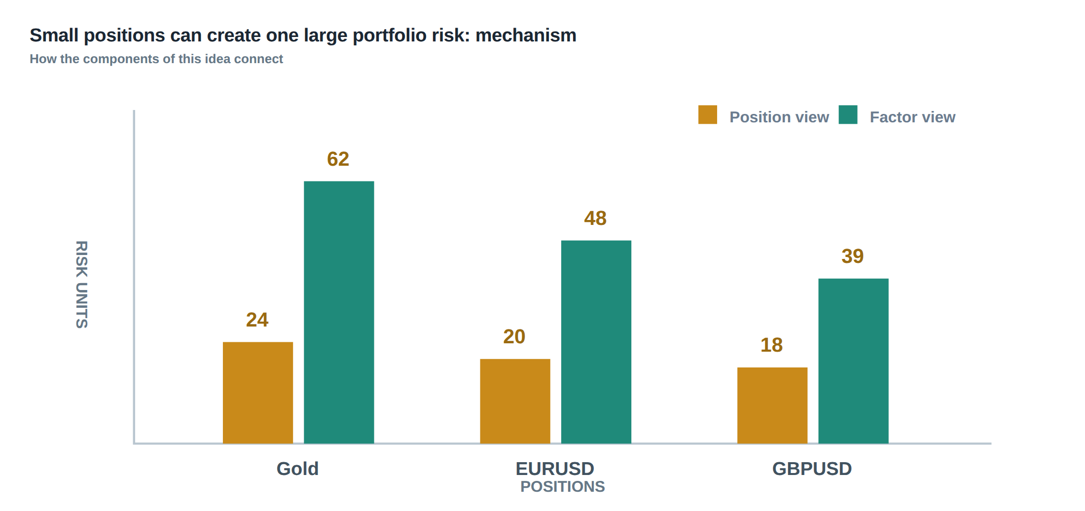
First, each trade is broken down into its factor sensitivities: delta to the underlying price, beta to a currency or index, duration to interest‑rate changes, and exposure to a volatility factor such as VIX or implied variance. These sensitivities are recorded in a factor‑exposure matrix that is updated in real time as positions are opened, closed, or re‑balanced.

Second, the matrix is multiplied by a covariance matrix of the underlying factors. The covariance matrix is built from a rolling window of high‑frequency returns, but it is also stress‑augmented with scenarios that inflate correlations during market dislocation – for example, a sudden 5 % move in the dollar index that historically coincides with a 30 % rise in equity volatility. The product yields a portfolio‑level variance and a set of “effective” exposures that are larger than the simple sum of the individual limits.

Third, the desk compares three exposure lenses: gross exposure (the absolute sum of all sensitivities), net exposure (gross minus offsetting positions), and stressed exposure (gross after applying the stressed covariance). If the stressed exposure breaches a pre‑defined factor‑level ceiling, the system flags the concentration even though each leg remains within its own limit. The flag triggers a mandatory review, a possible reduction of notional, or a hedge that directly targets the common factor.

A worked example with real numbers

Consider five long positions opened on the same day: a EUR/USD forward of €5 m, a S&P 500 futures contract worth $2 m, a 10‑year Treasury futures with a notional of $3 m, a crude‑oil ETF of $1 m, and a volatility swap paying the realised VIX squared on a $0.5 m notional. Individually each trade has a delta of roughly 0.2, a beta to the US dollar of 0.1, and a volatility exposure of 0.05, comfortably below a 2 % per‑trade limit set by the desk.

When the factor exposures are aggregated, the dollar beta sums to 0.5, the volatility beta to 0.25, and the combined delta to 1.0. Under normal market conditions the covariance between the dollar and VIX is modest (≈0.15), so the portfolio variance is acceptable. In a stress scenario where the dollar weakens by 4 % and VIX spikes by 25 % – a pattern observed in past risk‑on episodes – the correlation between the two jumps to 0.8. The stressed covariance matrix inflates the effective exposure to a delta of 3.2, a dollar beta of 2.0 and a volatility beta of 1.1. In other words, the five modest trades behave as if a single leveraged position with three times the original notional had been taken.

If the desk’s factor limit for dollar beta is 1.0, the stressed exposure exceeds it by 100 %. The risk manager must either unwind part of the portfolio, add a short dollar hedge of at least $6 m, or re‑allocate capital to a strategy with a negative dollar beta. The example illustrates that the “small‑position” myth collapses once common‑factor stress is introduced.

Where it breaks in live markets

The breakdown usually occurs when market participants collectively shift funding sources. During a sudden tightening of repo rates, the cost of financing the Treasury futures and the crude‑oil ETF rises in lock‑step, forcing both positions to move down as margin calls are met. The same liquidity squeeze also reduces the depth of the EUR/USD market, widening spreads on the forward and amplifying the dollar‑beta impact.

A second failure point is the assumption that correlations observed in calm periods persist. Empirical evidence shows that equity‑volatility, currency‑risk‑on, and credit‑spread correlations can double or triple in the first hour of a market shock. If the desk relies on a static correlation matrix, the stressed exposure will be severely underestimated, and the protective hedge will be undersized.

Finally, execution anomalies – such as a spike in order‑cancellation latency or a routing outage – can cause a cascade of stale orders. When the market moves quickly, a stale order that was meant to hedge the dollar exposure may be filled at an adverse price, turning a protective trade into a source of loss. The combination of factor stress and execution stress creates a perfect storm that overwhelms the individual‑limit framework.

The operating path, stage by stage

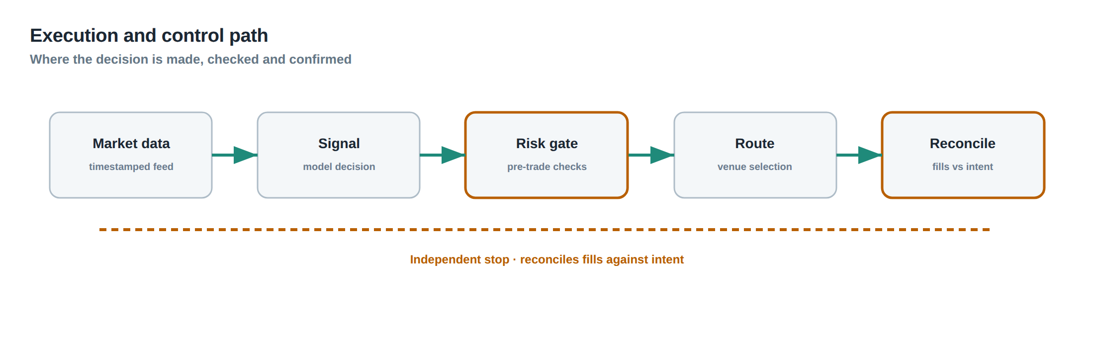
The first stage is data ingestion: market data, trade blotters, and funding rates are streamed into a central risk engine. The engine normalises the data to a common time‑grid and computes factor sensitivities for each new trade in real time.

The second stage is aggregation: the factor‑exposure matrix is summed across all open positions, and the current covariance matrix – both the baseline and the stress‑augmented versions – is applied. The engine outputs three exposure numbers for each factor: gross, net and stressed.

The third stage is policy enforcement: pre‑defined thresholds for each factor are checked against the three exposure numbers. If a stressed exposure breaches its limit, the system raises an alert that is routed to the desk head and the risk manager.

The fourth stage is response: the desk can automatically execute a hedge, reduce notional, or pause new submissions for the offending factor. The response logic is encoded in a workflow that records the decision, the rationale, and the time taken, creating an audit trail for post‑mortem analysis.

The final stage is feedback: the realised P&L from the hedge, the subsequent market moves, and any execution anomalies are fed back into the covariance estimator, allowing the stress scenarios to be refined for the next trading day.

Controls that act before the damage

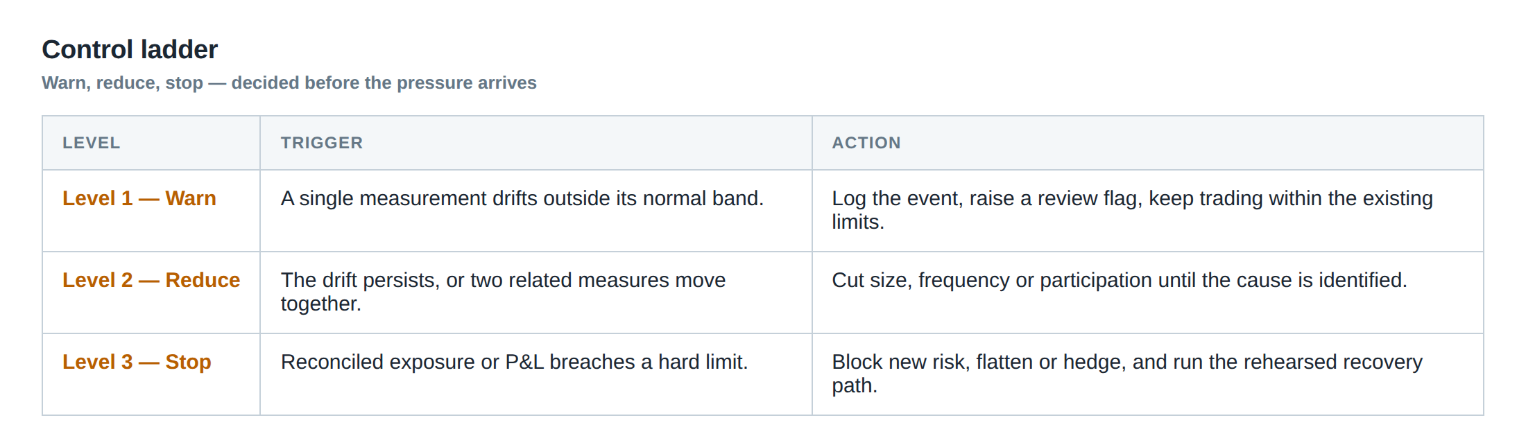
A ladder of controls is required to catch concentration before it materialises. The first rung is a pre‑trade check that calculates the incremental factor exposure of a proposed order and rejects it if the stressed exposure would exceed the limit. The second rung is a real‑time monitoring dashboard that displays the current stressed beta to the dollar, to volatility, and to funding spreads, colour‑coded by proximity to the limit.

The third rung is a periodic stress‑test run at the end of each trading session. The test re‑prices the entire portfolio under a set of extreme but plausible scenarios – a 5 % dollar move, a 30 % VIX jump, a 200 bp repo spike – and records the resulting stressed exposures. If any factor exceeds its threshold, a mandatory “risk‑reset” meeting is scheduled before the next market open.

The fourth rung is a post‑trade audit that reviews any order that was filled at a price outside the normal market depth, flagging it for a deeper investigation of execution latency and stale‑order frequency. By treating execution quality as part of the risk distribution, the desk ensures that tail‑risk from routing failures is captured in the same framework that captures factor stress.

How to measure whether it is working

Effectiveness is measured by comparing the realised tail loss distribution before and after the control suite is deployed. The key metric is the frequency of breaches of the stressed‑exposure limits; a reduction from, say, 12 breaches per month to fewer than two indicates that the pre‑trade checks are filtering out dangerous concentrations.

Another indicator is the average realised beta to the dollar during high‑volatility days. If the portfolio’s dollar beta, measured after hedges, stays within 0.3 of the target during periods when the dollar index moves more than 2 %, the stress‑adjusted limits are being respected.

A third, more subtle, measure is the “execution tail” – the proportion of orders that experience latency beyond the 95th percentile of the normal distribution. A falling execution tail, coupled with stable stressed exposure, suggests that the desk’s view of the loss distribution now incorporates both market and operational risk components.

The portfolio view

From a portfolio perspective the goal is to see the whole as less than the sum of its parts – not by naïve diversification, but by explicit factor de‑correlation. By maintaining a transparent map of how each strategy draws on shared liquidity pools, funding sources, and market‑wide risk factors, the desk can allocate capital to strategies that truly offset one another rather than merely appear small in isolation.

Gross exposure tells us how much notional is on the books, net exposure shows the offsetting positions, and stressed exposure reveals the hidden lever that emerges under duress. The three numbers together form a triad that must be monitored continuously. When the stressed exposure approaches the pre‑set ceiling, the portfolio manager must decide whether to add a true hedge – for example a short‑dollar future that directly reduces the dollar beta – or to rebalance the mix of strategies so that the common factor is no longer a single point of failure.

In practice, this approach forces the desk to ask a simple question for every new idea: “If the dollar were to move 4 % against the euro and VIX were to spike 20 % in the same minute, what would the portfolio’s loss look like?” The answer determines whether the idea passes the risk gate or needs to be reshaped.

Do you have a systematic process that quantifies the tail‑risk of factor‑linked concentration before a trade ever reaches the market?

About the research behind this lesson

Andrew Lo's lectures build risk analysis from return distributions and statistical measures, rather than treating one realised result as a complete description of risk.

Applied to this lesson: For a fast strategy, median latency or average fill quality is not enough. The review has to include tail delays, stale-order frequency and the loss distribution when cancellation or routing behaves abnormally.

Two live systems, one desk

PULSE-X — power-packed HFT: high-frequency momentum on XAUUSD and EURUSD. System details · Live account

NIC-X — ultra-low drawdown: displaced-print arbitrage for large capital. System details · Live account

Start now: leave your email and request a free trial — we will send the pricing, the connection route and the trial terms. Pricing

Join the market discussion: Telegram @squawklive

Source: Risk and Return

Educational content only. Trading leveraged products involves risk.