November 7, 2026

What this problem really is

The phrase “one lot” is often taken to mean a fixed monetary exposure – for example, a standard futures contract representing $50 000 of notional. In practice the risk that a trader actually bears from that lot is a function of how far the price moves, and price movement is not constant. When the underlying’s typical volatility expands, the same lot can generate twice the profit‑and‑loss swing, and consequently twice the capital that must be set aside to meet a pre‑agreed risk budget. The problem is therefore one of unstable risk: a static position size hides a dynamic exposure that can breach limits in a matter of minutes.

If the desk allocates a fixed 1 % of equity to each trade, the calculation of how many contracts to buy must incorporate an estimate of the instrument’s future volatility. When that estimate changes, the “one lot” definition changes in practice, even though the contract specifications have not. The mismatch becomes acute for high‑frequency or intraday strategies that rebalance many times a day; a sudden surge in realised volatility can turn a modest‑sized order into a tail‑risk event.

The issue is not merely academic. During the 2020 market stress, many statistical arbitrage desks discovered that their daily VaR calculations, which assumed a 20‑day historical volatility, were dramatically under‑estimating the true risk because the realised intraday volatility had doubled. The consequence was a cascade of margin calls that forced rapid deleveraging. The root cause was the assumption that a “lot” carried a constant risk weight, an assumption that collapses the moment the volatility regime shifts.

How the mechanism works, step by step

The first step is to obtain a forward‑looking volatility estimate. Most desks use an exponentially weighted moving standard deviation of recent returns, typically over a look‑back of 30 to 120 minutes for intraday signals. The choice of window is a trade‑off: a short window reacts quickly to spikes but produces noisy size adjustments; a long window smooths noise but lags the true market state.

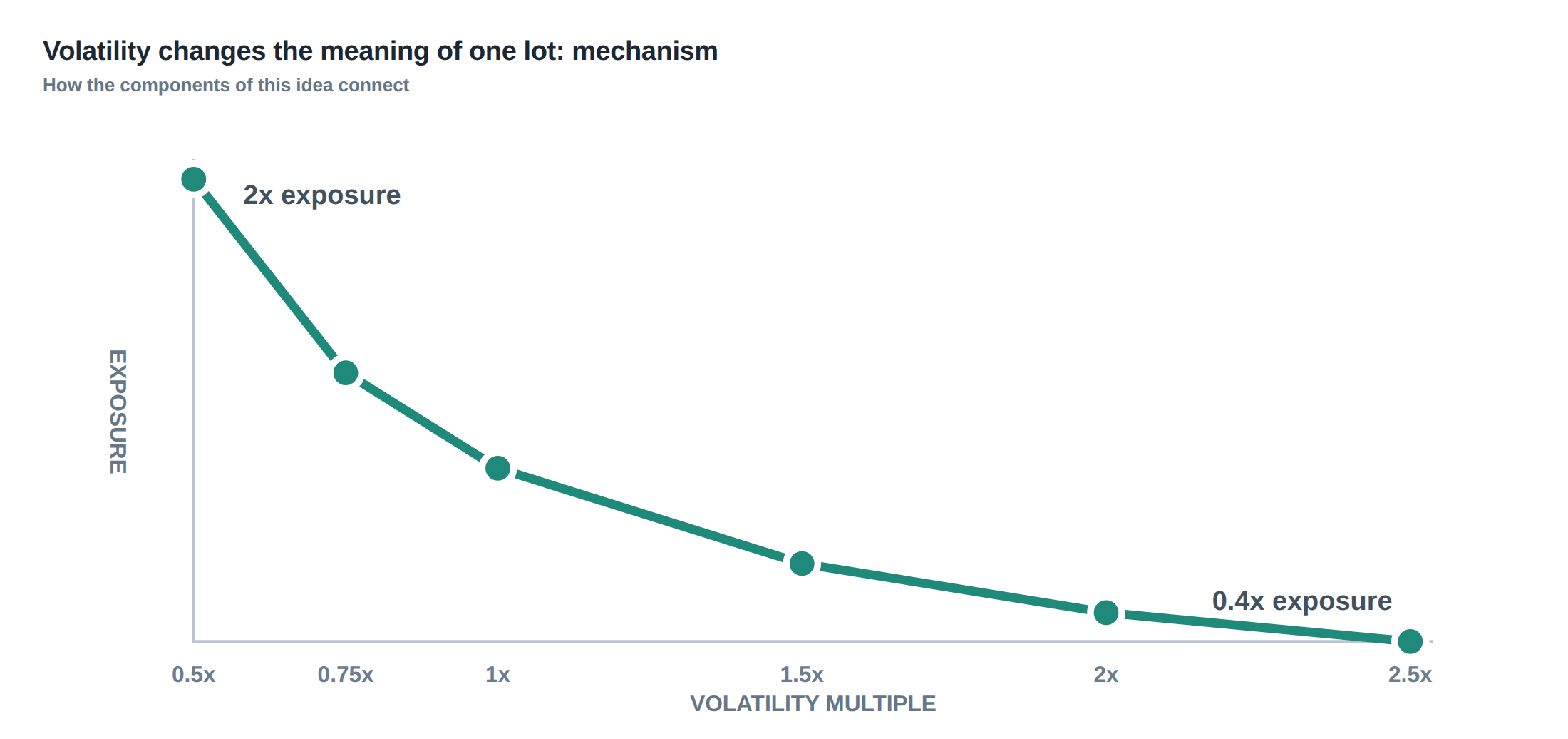
Once the volatility σ̂ is calculated, the desk defines a volatility‑scaled lot size L = (R / σ̂) × K, where R is the risk budget per trade expressed as a proportion of equity, and K is a scaling constant that converts the dimensionless ratio into a contract count. The inverse‑volatility rule ensures that if σ̂ doubles, L halves, keeping the product σ̂ × L roughly constant.

A second step introduces hard limits: a floor on σ̂ to prevent the denominator from collapsing to zero during tranquil periods, and a cap on L to stop the system from allocating an impractically large number of contracts when volatility is extremely low. These bounds act as a safety ladder that keeps the algorithm within operational constraints, regardless of statistical outliers.

Finally, the algorithm monitors market microstructure signals – order‑book depth, latency spikes, and stale‑quote frequencies – to decide whether to suspend the scaling rule. In markets that are fragmented, illiquid, or experiencing a discontinuity (for example, after a circuit‑breaker reset), the volatility estimate may be unreliable, and the system should revert to a conservative flat size or pause trading entirely.

A worked example with real numbers

Assume the desk trades a Euro‑Stoxx 50 futures contract, each representing €10 million of notional. The equity allocated to the strategy is €20 million, and the risk budget per trade is set at 0.5 % of equity, i.e. €100 000. The current volatility estimate, derived from the last 60 minutes of 1‑minute returns, is 12 % annualised, which translates to a 0.6 % intraday standard deviation (≈ σ̂ = 0.006).

Applying the inverse‑volatility rule, the raw lot factor is R / σ̂ = 100 000 / 0.006 ≈ 16 666 667. Dividing by the contract’s price sensitivity – a €10 million contract moves roughly €100 per tick – yields a base size of about 167 contracts. The desk imposes a floor σ̂ = 0.004 (corresponding to a 8 % annualised volatility) and a cap of 200 contracts. In this calm scenario the calculated size of 167 contracts sits comfortably within the limits.

Now suppose a sudden macro news release pushes the realised volatility estimate to 24 % annualised, i.e. σ̂ = 0.012 for the same 60‑minute window. The inverse‑volatility factor becomes 100 000 / 0.012 ≈ 8 333 333, halving the raw contract count to roughly 84 contracts. Because the risk budget has not changed, the exposure measured in € per tick is now half of the previous level, exactly as the rule predicts.

If the volatility estimate were to spike to 48 % annualised (σ̂ = 0.024), the algorithm would compute a size of about 42 contracts. The floor on σ̂ prevents the denominator from falling below 0.004, but the cap on contracts is never triggered because the size is already well below the upper bound. The example demonstrates how a doubling of σ̂ directly halves the position, preserving the intended risk budget even as market turbulence varies dramatically.

Where it breaks in live markets

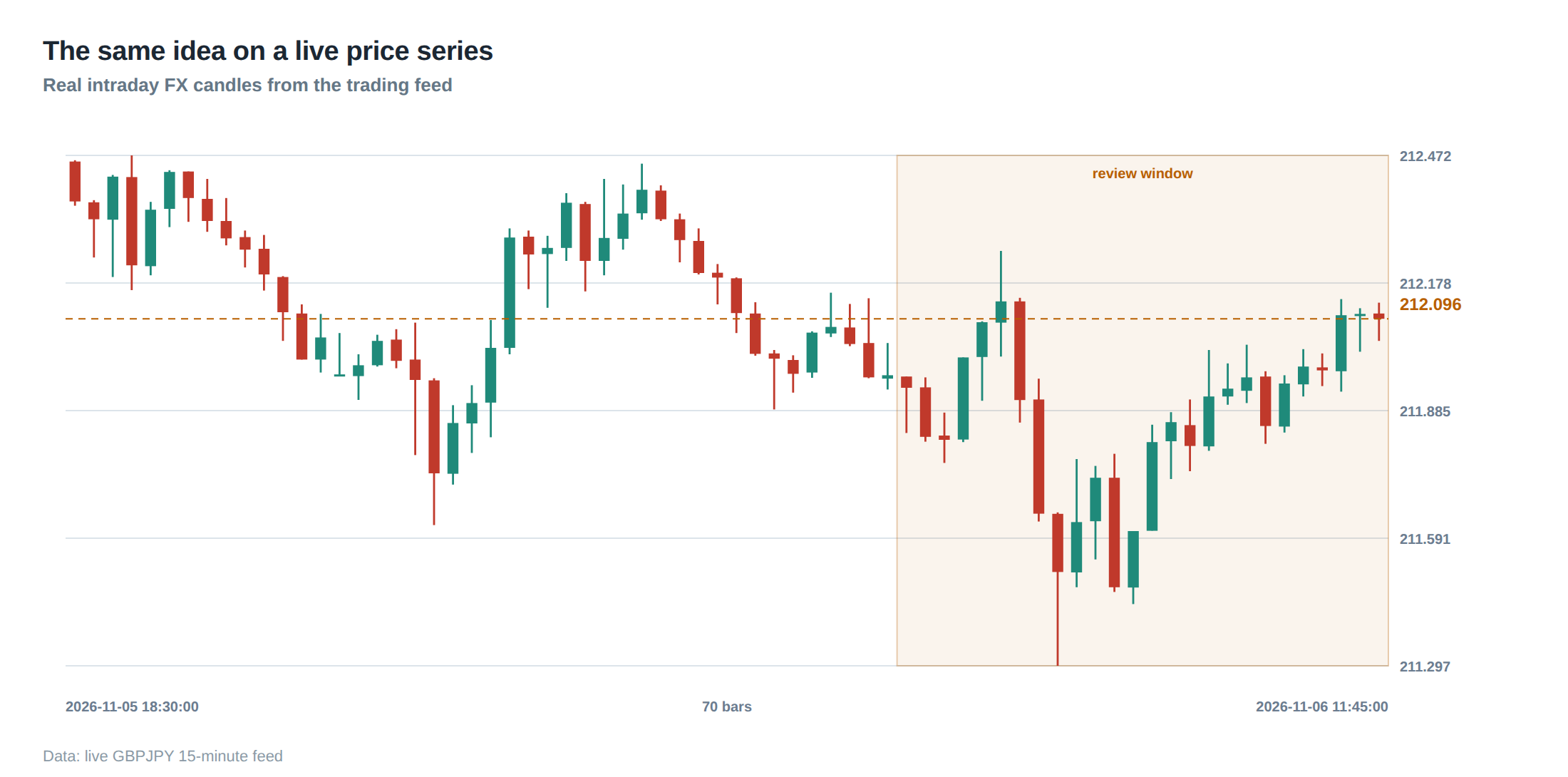
The elegance of the inverse‑volatility rule collapses when the volatility estimator itself becomes corrupted. In fragmented electronic markets, a single venue may experience a temporary outage, causing a burst of zero‑return bars that artificially depress σ̂. The algorithm, seeing a low volatility, would then inflate the lot size, exposing the desk to a hidden concentration risk that only materialises when the venue recovers and price discovery resumes.

Another failure mode occurs during discontinuous price jumps, such as those caused by circuit‑breaker releases or large block trades that clear multiple levels of the order book in one millisecond. The statistical estimator, which assumes a continuous diffusion, will interpret the jump as a temporary volatility spike and immediately shrink the position. If the trader is already long a sizeable order, the abrupt reduction can lead to forced liquidations at unfavourable prices, especially if the market depth is thin.

Latency anomalies also undermine the mechanism. If the execution platform suffers a median latency increase from 150 µs to 500 µs, the realised P&L distribution widens, but the volatility estimator – which looks at price changes – may not capture the delay‑induced slippage. Consequently, the risk model under‑estimates the true exposure, and the “one lot” definition becomes a mis‑statement of the actual capital at risk.

Finally, the rule assumes that the risk budget R is static. In practice, desk‑level capital allocations can be altered by overnight P&L, margin calls, or strategic re‑balancing. If R is reduced while σ̂ remains low, the algorithm may still generate a size that violates the new, tighter capital constraint, because the scaling factor does not automatically incorporate changes in the denominator beyond volatility.

The operating path, stage by stage

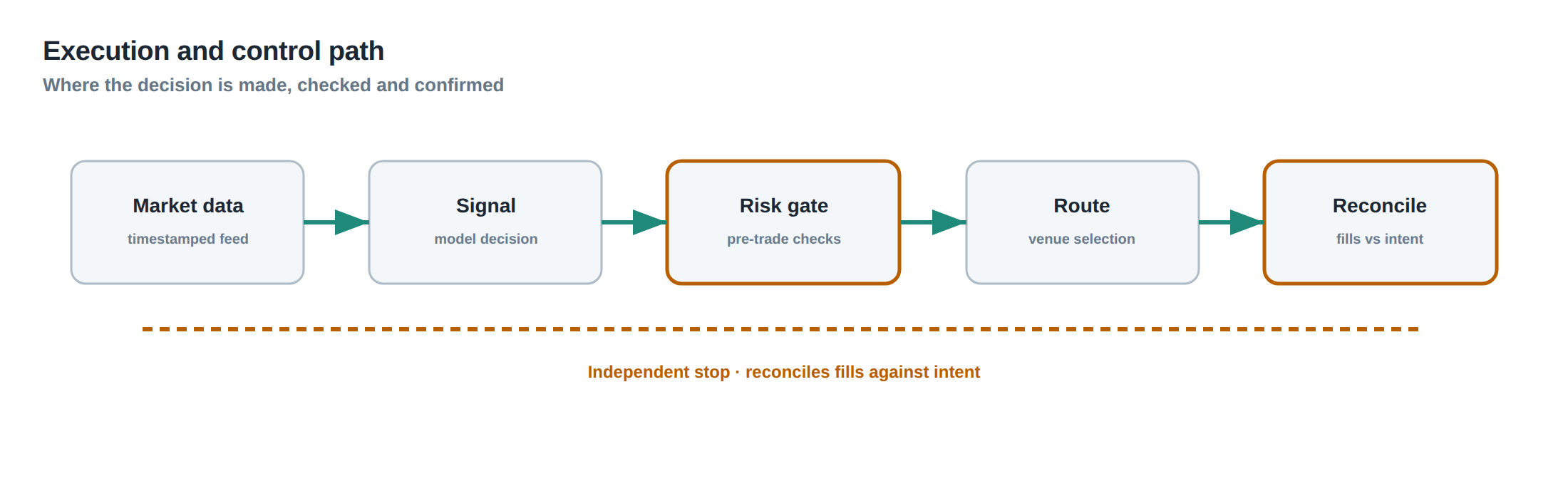
The first stage is data acquisition: high‑frequency price ticks, order‑book snapshots, and latency metrics are streamed into a rolling buffer. The buffer is segmented into overlapping windows that feed the volatility estimator, which updates every minute. The second stage computes the raw lot factor using the inverse‑volatility formula, then applies the pre‑defined floor and cap.

The third stage is a market‑state filter. It examines microstructure health indicators – such as the proportion of stale quotes, the frequency of rejected orders, and the variance of fill prices – to decide whether the volatility‑scaled size should be accepted, reduced, or discarded. If the filter flags an abnormal state, the system either reverts to a flat size (e.g., a fixed 50 contracts) or pauses trading for a configurable cool‑down period.

The fourth stage is order generation. The chosen size is translated into a set of limit and market orders that respect venue‑specific minimum tick sizes and lot increments. Risk checks at this point verify that the aggregate exposure across all instruments remains within the global VaR and stress‑test limits.

The final stage is post‑trade monitoring. Realised P&L, execution quality, and the deviation between predicted and observed volatility are logged. These data feed back into the next iteration of the volatility estimator, closing the loop and allowing the system to self‑correct over time.

Controls that act before the damage

A multi‑layered control architecture is essential to prevent the volatility‑scaled lot from becoming a source of loss. The first layer is the statistical guardrail: the volatility floor and contract cap are hard‑coded constants that cannot be overridden by the live algorithm, ensuring that extreme parameter values are never passed to the order engine.

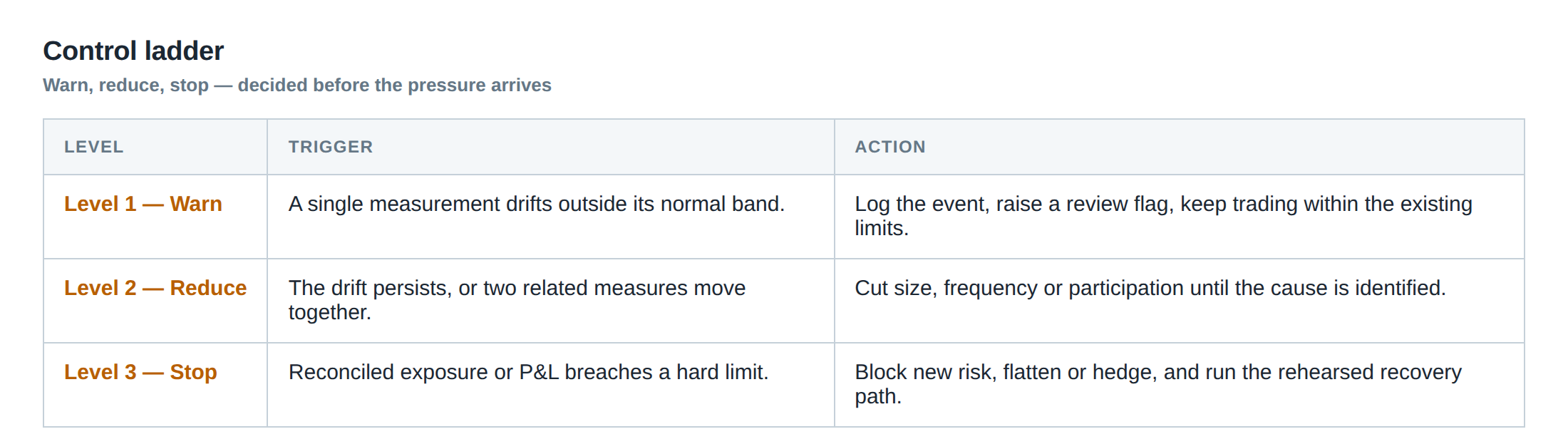
The second layer is the microstructure health monitor. It continuously computes a composite health score from latency, fill‑rate, and stale‑order metrics. When the score falls below a threshold, the system automatically reduces the target size by a pre‑specified factor (for example, 30 %) or switches to a flat‑size mode. This pre‑emptive reduction limits exposure before a potential market breakdown translates into realised loss.

The third layer consists of a capital‑allocation watchdog. It watches the desk’s available margin and the cumulative risk budget across all active strategies. If the aggregate risk utilisation exceeds a configured percentage (say 80 %), the watchdog throttles new position initiations, regardless of the volatility estimate.

The fourth layer is a manual override panel. Senior traders can intervene to pause or adjust the volatility scaling parameters in response to news events that the automated system cannot anticipate, such as central‑bank announcements or geopolitical shocks. The override is logged with a timestamp and justification, providing an audit trail for later review.

Together these controls create a ladder of protection: statistical limits stop the algorithm from proposing absurd sizes, health monitors catch deteriorating market conditions, capital watchdogs enforce portfolio‑level discipline, and human oversight adds a final safety net.

How to measure whether it is working

Effectiveness is judged by comparing the realised risk of the volatility‑scaled positions against the intended risk budget. One metric is the ex‑post standard deviation of P&L per trade, expressed as a percentage of equity; it should stay close to the pre‑defined R, typically within a 10 % tolerance band.

Another useful indicator is the size‑adjustment lag: the number of minutes between a significant change in realised volatility (for example, a 20 % jump) and the corresponding change in contract size. A lag longer than the chosen look‑back window suggests that the estimator is not responsive enough, while a lag shorter than the market’s natural reaction time may indicate over‑fitting to noise.

Execution quality provides an indirect measure. If the average slippage per contract remains stable across volatility regimes, it implies that the size scaling is not forcing the algorithm into illiquid price levels. Conversely, a rising slippage trend when volatility spikes signals that the floor/cap limits are being breached or that the health filter is not acting swiftly enough.

Finally, stress‑test results – simulated runs where volatility is artificially inflated to extreme levels – should show that the maximum exposure never exceeds the predetermined capital ceiling. By logging the highest realised exposure during these tests and comparing it with live‑trading peaks, the desk can confirm that the control ladder is functioning as designed.

The portfolio view

From a portfolio perspective, each instrument’s volatility‑scaled lot contributes to a matrix of covariances that determines the overall portfolio VaR. Because the lot size is inversely proportional to σ̂, the contribution of a high‑volatility asset to portfolio variance is intentionally dampened, while low‑volatility assets receive a modest size boost. This dynamic rebalancing tends to equalise risk contributions across the basket, a property known as risk parity at the contract level.

However, the approach also introduces a hidden correlation: when market stress lifts volatilities across many assets simultaneously, the algorithm reduces all positions, potentially pulling the portfolio out of the market at the worst possible moment. To mitigate this, the desk may overlay a minimum exposure rule that guarantees a baseline participation in each asset, preserving diversification benefits even during systemic spikes.

The portfolio manager must also monitor the aggregate turnover generated by the scaling rule. Frequent size adjustments increase transaction costs and can erode the edge of a high‑frequency strategy. By selecting a look‑back that balances responsiveness with turnover, the desk can keep the annualised turnover at a target level (for example, 30 % of notional) while still reacting to genuine regime changes.

In practice, the portfolio’s realised Sharpe ratio, after accounting for scaling‑induced turnover and slippage, serves as the ultimate performance gauge. If the Sharpe remains stable or improves when volatility regimes shift, the volatility‑scaled lot methodology can be deemed successful. If, however, the Sharpe collapses during turbulent periods, the desk should revisit the look‑back, floor, cap, or health‑filter parameters.

Is your current lot‑sizing framework truly insulated from the volatility regime shifts that dominate modern markets?

About the research behind this lesson

Andrew Lo's lectures build risk analysis from return distributions and statistical measures, rather than treating one realised result as a complete description of risk.

Applied to this lesson: For a fast strategy, median latency or average fill quality is not enough. The review has to include tail delays, stale-order frequency and the loss distribution when cancellation or routing behaves abnormally.

Two live systems, one desk

PULSE-X — power-packed HFT: high-frequency momentum on XAUUSD and EURUSD. System details · Live account

NIC-X — ultra-low drawdown: displaced-print arbitrage for large capital. System details · Live account

Start now: leave your email and request a free trial — we will send the pricing, the connection route and the trial terms. Pricing

Join the market discussion: Telegram @squawklive

Source: Risk and Return

Educational content only. Trading leveraged products involves risk.