November 7, 2026

What this problem really is

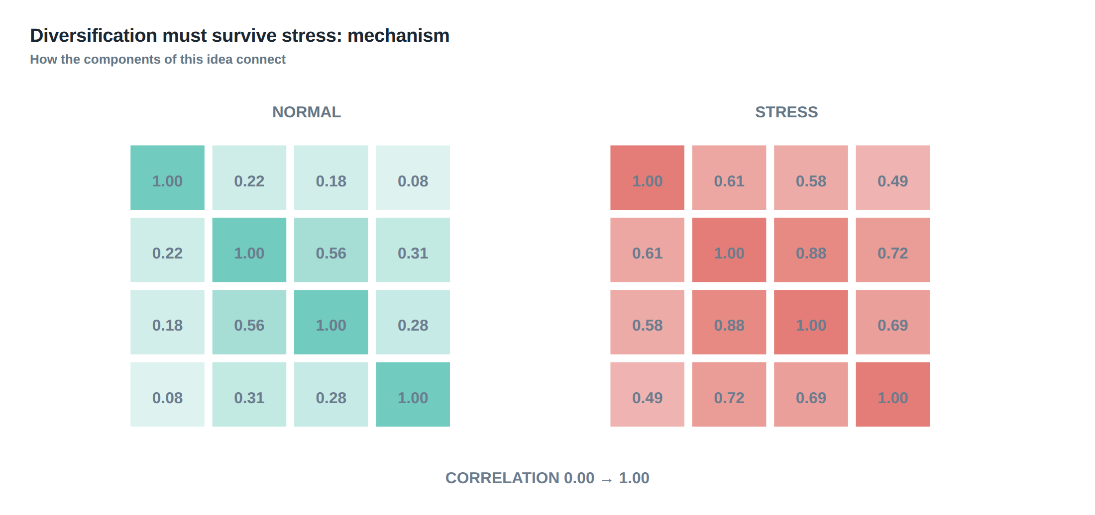
The intuition that a portfolio of low‑correlated strategies is automatically safe is a relic of calm‑market thinking. In normal conditions the Pearson correlation between a statistical arbitrage pair‑trade and a macro‑driven carry strategy may sit comfortably at 0.15, suggesting that a joint loss is unlikely. Yet the same statistical relationship is a conditional expectation: it assumes the market environment that generated the data continues to hold. When liquidity dries, funding costs spike, or a systemic shock forces a mass margin call, the underlying drivers of those returns can align, turning an apparently diversified book into a single‑point failure.

The problem is therefore not a lack of correlation per se, but the fragility of the correlation estimate itself. Correlation matrices built on a rolling three‑month window of 5‑minute returns will capture the typical co‑movement of price and spread, but they ignore the tail dependence that appears when risk limits are breached. In the tail, the joint distribution collapses onto a lower‑dimensional manifold defined by shared funding constraints, common order‑book depth, and the collective reaction of market participants to a rapid price move. The diversification that survived the last quarter may evaporate in the next stress episode.

A second, often hidden, dimension is the liquidity‑adjusted concentration of the portfolio. Two strategies that appear uncorrelated in price may both rely on the same pool of high‑frequency market‑making capacity. When that capacity is withdrawn—whether by a regulator tightening order‑to‑trade ratios or by a large dealer reducing its balance‑sheet exposure—both strategies experience a simultaneous widening of execution costs. The loss is not captured by a simple correlation coefficient but by a concentration measure that weights each strategy’s exposure to a common liquidity factor.

The core thesis, therefore, is that relationships estimated in normal markets can change precisely when risk limits matter most. The practitioner must build a stress‑aware view of correlation, factor exposure, and liquidity concentration, and must set limits before those relationships break down.

How the mechanism works, step by step

The first step is to construct a baseline correlation matrix from a representative sample of returns, typically using a rolling window that balances statistical significance against regime shift. From this matrix we extract the principal components that explain the bulk of variance; the first few components often correspond to market‑wide factors such as equity index moves, implied volatility, or funding spreads.

Next we generate a set of stress scenarios that target the same factors but with magnitudes observed during historical crises—e.g., a 300 bp jump in overnight repo rates, a 40 % drop in order‑book depth, or a 2‑sigma increase in realised volatility across all asset classes. For each scenario we apply a factor shock to the baseline matrix, recomputing the implied correlations under the new factor loadings. This produces a stressed correlation matrix that reflects how co‑movements are likely to evolve when the factors move together.

A parallel exercise is to model the simultaneous widening of spreads and expansion of volatility. Using a GARCH‑type volatility model calibrated to the same historical window, we impose a volatility shock that raises the conditional variance of each instrument by a predetermined factor. At the same time we increase the bid‑ask spread for each venue by a percentage proportional to the liquidity shock. The joint impact on expected transaction costs and execution risk is then fed back into the correlation calculation, because higher costs tend to reduce the effective position size and alter the risk‑adjusted return profile.

The third step introduces crowd‑exit dynamics. When a large participant—often a dealer or a high‑frequency market‑maker—exits a market, the remaining participants experience a surge in margin calls as the price impact of their orders grows. We model this by adding a binary “crowded‑exit” variable that, when triggered, multiplies the margin‑requirement vector for all strategies that share the same funding source. The result is a correlated increase in capital utilisation across the portfolio, which in turn raises the probability of hitting pre‑set risk limits simultaneously.

Finally, we recompute a liquidity‑adjusted concentration metric. Rather than the naïve Herfindahl index on notional, we weight each strategy’s notional by its marginal impact on market depth under the stressed scenario. The concentration score therefore rises sharply when several strategies depend on a thin slice of the order book that is simultaneously stressed. This score is the quantitative trigger for tightening diversification limits.

A worked example with real numbers

Consider two systematic strategies running on the same prop desk: Strategy A is a statistical arbitrage pair‑trade on US equity futures, and Strategy B is a carry trade that exploits the cross‑currency basis between EUR/USD and GBP/USD. Over the past twelve months the daily returns of A and B have an empirical correlation of 0.12, and their individual Sharpe ratios are 1.8 and 2.1 respectively. The desk’s risk model shows a liquidity‑adjusted concentration of 0.18, comfortably below the internal threshold of 0.30.

In the stress test we impose a 250 bp shock to overnight funding rates, a 35 % reduction in depth on the primary CME order book, and a 1.5‑times increase in realised volatility for all equity futures. The factor loadings for both strategies on the funding factor rise from 0.05 to 0.42, while their loadings on the depth factor move from 0.03 to 0.38. Re‑computing the correlation under these new loadings yields a stressed correlation of 0.68, a more than five‑fold increase.

Simultaneously, the widened spreads raise the average execution cost for Strategy A from 0.8 bps to 3.2 bps per trade, and for Strategy B from 0.5 bps to 2.0 bps. The higher costs cut the effective Sharpe ratios to 0.9 and 1.1 respectively. Because both strategies now require roughly double the capital to maintain the same risk‑adjusted exposure, the liquidity‑adjusted concentration rises to 0.42, exceeding the desk’s limit.

If a crowded exit is triggered—say a major dealer withdraws 30 % of its market‑making capacity in the CME futures market—the margin requirement multiplier for both strategies jumps to 1.35. The combined effect pushes the portfolio’s aggregate VaR from 1.2 % of capital to 2.5 % in a single day, breaching the 2 % daily VaR limit. The example demonstrates that despite a low historical correlation, the two strategies can lose together when they share liquidity and funding dependencies that are exposed under stress.

Where it breaks in live markets

In live trading the first point of failure is often the latency of the execution engine. Under normal conditions a median round‑trip time of 150 µs is acceptable, but during a market‑wide surge in order flow the same infrastructure may experience tail latencies of several milliseconds. Those tail events are not captured by the median latency metric, yet they are precisely the moments when a crowded exit can cause a cascade of stale orders and missed fills.

A second failure mode is the assumption that fill quality remains stationary. When a liquidity shock hits, the probability of a price‑improving fill drops dramatically, and the proportion of orders that are cancelled after being partially filled spikes. The loss distribution for a strategy that relies on tight spreads therefore develops a heavy left tail, which is invisible to a simple standard‑deviation‑based risk model.

Third, the risk limits themselves can become self‑fulfilling. If a strategy’s position limit is defined relative to a moving average of daily turnover, a sudden drop in turnover due to market stress will tighten the limit in real time, forcing the trader to unwind positions at the same time as others are doing the same. The resulting synchronised exit amplifies price impact, widens spreads further, and pushes the correlation to its stressed value.

Finally, the data feed integrity can degrade. In a high‑frequency environment a single missed quote or an out‑of‑sync timestamp can cause the downstream correlation estimates to be based on mismatched time series, producing spurious low‑correlation readings that disappear as soon as the feed recovers. The moment of recovery is often when the portfolio is already exposed to the stressed correlation structure.

The operating path, stage by stage

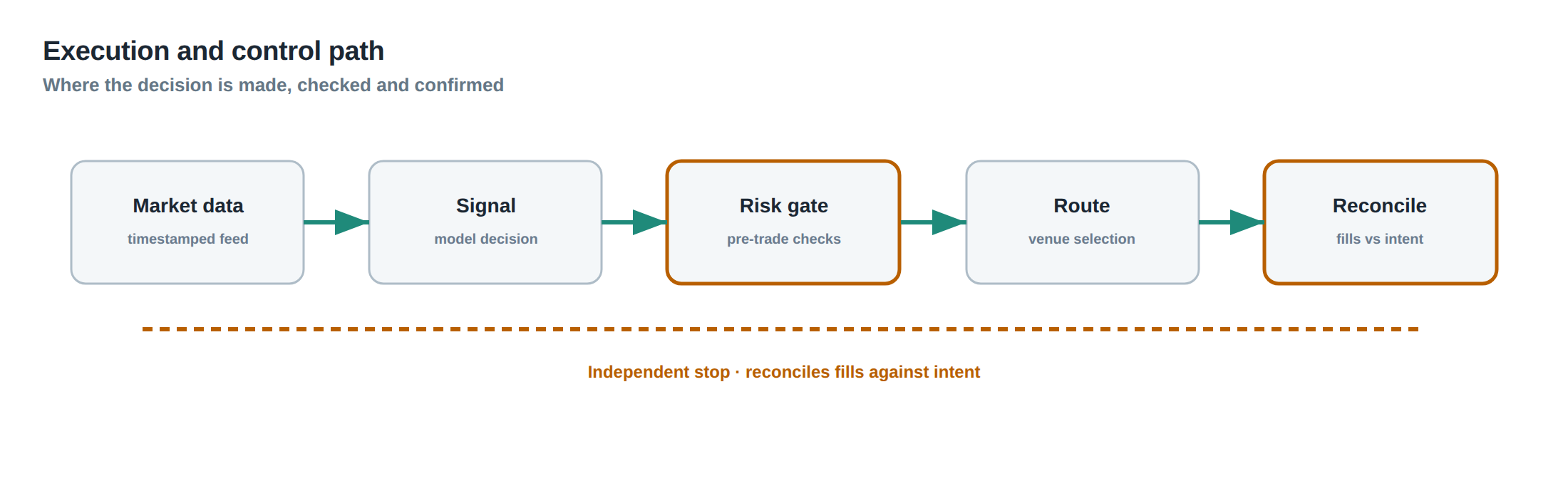
The first stage is data ingestion, where raw tick data are normalised and aligned to a common timestamp grid. At this point the system calculates the baseline covariance matrix and extracts factor loadings using a principal‑component analysis. The second stage introduces the stress overlay: a library of factor shock vectors is applied to the baseline loadings, and a stressed covariance matrix is recomputed in real time.

The third stage evaluates the liquidity‑adjusted concentration. For each strategy the system estimates marginal market impact under the stressed depth scenario, then aggregates the weighted notional exposures to produce a concentration score. If the score exceeds a predefined threshold, the system flags the portfolio for review.

The fourth stage simulates simultaneous spread widening and volatility expansion. Using a calibrated GARCH model, the system inflates the conditional variance and spreads, recomputes expected transaction costs, and adjusts the Sharpe estimates for each strategy. The resulting risk‑adjusted returns feed into a VaR calculator that incorporates the crowd‑exit multiplier when a funding‑source stress is detected.

The final stage is the limit enforcement engine. It compares the stressed VaR, concentration score, and individual strategy Sharpe ratios against the desk’s risk limits. If any metric breaches its limit, the engine automatically reduces position sizes, raises margin requirements, or temporarily disables new order entry for the affected strategies. The entire pipeline runs on a sub‑second cycle, ensuring that the diversification assessment reflects the most recent market conditions.

Controls that act before the damage

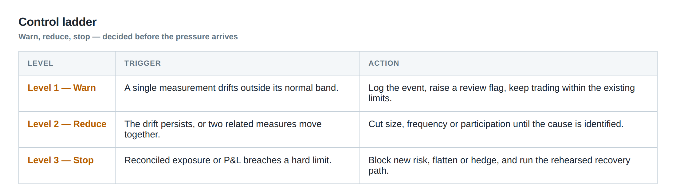
A pre‑trade control checks the current liquidity‑adjusted concentration against the limit before allowing a new order. If the addition would push the score above 0.30, the order is rejected or scaled down. A post‑trade control monitors realised spread widening; when the realised spread exceeds 2.5 times the historical average for a given venue, the system raises an alert and temporarily reduces the order‑size cap for all strategies that share that venue.

A separate margin‑call monitor watches the funding‑rate factor. When the overnight repo rate moves more than 150 bp from its 30‑day average, the monitor applies a margin‑requirement multiplier to any strategy with a loading above 0.3 on that factor. This multiplier is reflected in the VaR calculation, ensuring that capital allocation is tightened before the portfolio breaches its daily loss limit.

Liquidity‑stress tests are run daily at market close. The test re‑runs the entire stress‑scenario pipeline with the most recent data, producing a “stress‑gap” report that quantifies the difference between normal‑market and stressed‑market correlation, VaR, and concentration. If the stress‑gap exceeds a predefined tolerance—e.g., a VaR increase of more than 80 %—the desk must rebalance the portfolio or raise capital before the next trading day.

Finally, a “crowded‑exit” detector analyses order‑book depth across all venues in real time. When the aggregate depth on a venue falls below 5 % of its 30‑day average for more than five minutes, the detector flags a potential exit scenario. The flag triggers an immediate reduction in position limits for any strategy that sources liquidity from that venue, preventing a cascade of forced liquidations.

How to measure whether it is working

The primary performance indicator is the realised stress‑gap. After each trading day the desk calculates the realised VaR under the actual market conditions and compares it to the stressed VaR that was forecast at the start of the day. The ratio of realised to stressed VaR should stay below one; a systematic overshoot indicates that the stress model is under‑estimating tail dependence.

A second indicator is the frequency of limit breaches caused by the concentration score. If the number of times the liquidity‑adjusted concentration exceeds its threshold rises, it suggests that the underlying factor shocks are becoming more correlated than the model assumes, and the stress scenarios need to be recalibrated.

Third, the tail‑latency distribution of the execution engine is monitored. The 99.9 th percentile of round‑trip latency must remain within the pre‑defined bound (e.g., 2 ms). An upward drift in this percentile is a leading indicator of a forthcoming degradation in fill quality, which in turn can inflate the realised spread and push the portfolio toward the stressed correlation regime.

Finally, the desk tracks the “crowded‑exit” trigger count. A rising count over a rolling window signals that market‑making capacity is being withdrawn faster than anticipated, and the stress‑scenario library should be expanded to include larger funding‑rate shocks or deeper spread expansions.

The portfolio view

When the stress‑aware framework is applied, the portfolio is no longer a simple list of pairwise correlations but a multidimensional surface that reacts to factor shocks, liquidity withdrawals, and margin‑call cascades. The surface is characterised by three axes: (i) the stressed correlation matrix, (ii) the liquidity‑adjusted concentration, and (iii) the volatility‑spread envelope. A point on this surface represents the portfolio’s risk state under a particular combination of factor values.

In practice the desk visualises this surface as a heat map, with colour intensity indicating the magnitude of VaR. Regions of high intensity correspond to scenarios where the correlation has inflated, spreads have widened, and concentration has risen—precisely the conditions under which diversification disappears. By overlaying the current market point on this map, traders can see how close they are to a dangerous region and can act pre‑emptively.

The key operational insight is that diversification is a dynamic property, not a static label. A portfolio that appears well‑diversified today may sit on the edge of a high‑VaR region tomorrow if funding conditions deteriorate or a major dealer exits. The continuous stress‑testing pipeline, together with the pre‑trade and post‑trade controls, ensures that the desk maintains a margin of safety that is measured in real‑time, rather than relying on historical averages that become meaningless when the market is under stress.

Is your current diversification framework capable of detecting the moment when the very relationships you rely on begin to unravel?

About the research behind this lesson

Andrew Lo's lectures build risk analysis from return distributions and statistical measures, rather than treating one realised result as a complete description of risk.

Applied to this lesson: For a fast strategy, median latency or average fill quality is not enough. The review has to include tail delays, stale-order frequency and the loss distribution when cancellation or routing behaves abnormally.

Two live systems, one desk

PULSE-X — power-packed HFT: high-frequency momentum on XAUUSD and EURUSD. System details · Live account

NIC-X — ultra-low drawdown: displaced-print arbitrage for large capital. System details · Live account

Start now: leave your email and request a free trial — we will send the pricing, the connection route and the trial terms. Pricing

Join the market discussion: Telegram @squawklive

Source: Risk and Return

Educational content only. Trading leveraged products involves risk.