November 8, 2026

What this problem really is

A draw‑down, in the simplest sense, is the distance between a strategy’s historical peak equity and the subsequent trough before a new peak is established. At a prop desk the figure is usually reported as a percentage of the allocated capital, but the raw number tells us little about the health of the underlying process. Without a disciplined response plan the draw‑down becomes a passive statistic – a historical footnote that does not influence future behaviour. In practice the danger lies not in the loss itself but in the temptation to “make it up” by increasing exposure, a reaction that is rarely justified by the data that produced the loss.

Two dimensions are required to make the metric useful. First, the measurement must be performed at both the individual strategy level and the aggregated portfolio level, because a single systematic loss can be masked by unrelated winners if only the portfolio figure is watched. Second, the measurement must be coupled to a set of pre‑defined actions – warnings, de‑risking steps, and, if necessary, a complete shutdown. When the thresholds are hard‑wired into the execution engine, the draw‑down ceases to be a passive observation and becomes a trigger for a controlled recovery process.

The importance of this coupling is underlined by the statistical nature of trading returns. Return distributions are heavy‑tailed; a single extreme loss does not represent the expected behaviour of the strategy. Treating that loss as the sole descriptor of risk is equivalent to assuming the entire distribution collapses to a point. The literature on risk analysis emphasises that a robust risk framework must consider the full distribution – median latency, average fill quality, and, crucially, the tail of latency, stale‑order frequency and loss outcomes when execution deviates from the norm. Only by embedding those tail‑risk considerations into a draw‑down control can a desk protect optionality and avoid the cascade that follows an unchecked loss.

How the mechanism works, step by step

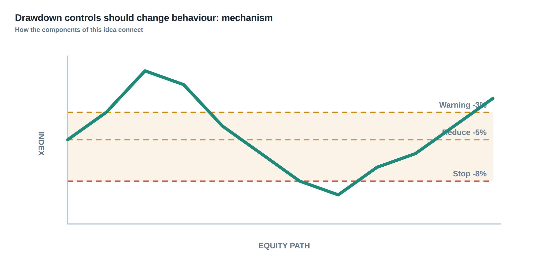
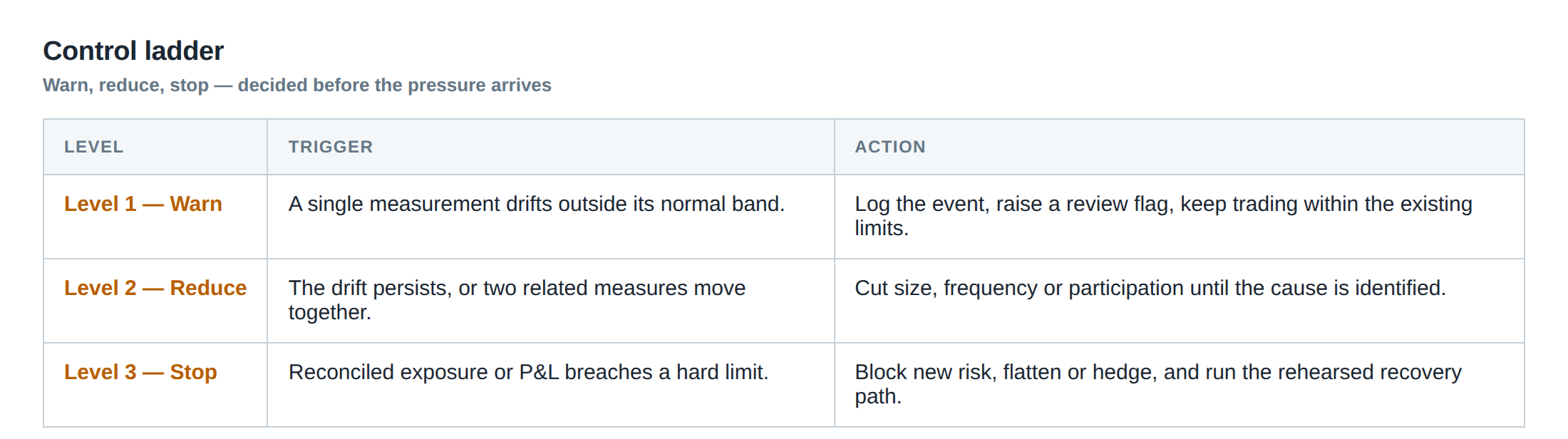
The first step is to define a peak‑to‑trough metric for each strategy. The system records the highest equity level achieved since the last reset, then continuously monitors the current equity. When the current equity falls below a pre‑set proportion of the peak – for example 5 % – a warning flag is raised. The warning does not alter position sizing; it simply alerts the risk team and logs the event for later analysis.

If the equity continues to erode and breaches a second, tighter threshold – say 10 % – the de‑risking routine is invoked. De‑risking can take several forms: halving the notional exposure, tightening the stop‑loss band, or moving the strategy to a lower‑frequency execution mode. The key is that the reduction is automatic and does not require a discretionary decision at the moment of loss, thereby removing emotional bias.

Should the equity fall to a third, critical level – for instance 15 % – the system initiates a shutdown. All open orders are cancelled, positions are liquidated according to a pre‑approved unwind schedule, and the strategy is marked inactive until a post‑mortem is completed and a risk committee signs off on a re‑activation plan. The shutdown threshold is deliberately set below the level at which the desk would normally consider “recovering” the loss by adding capital, because the latter behaviour has been shown to convert a model misspecification into ruin.

A final, often overlooked, component is the time‑under‑water metric. Two strategies may each suffer a 10 % draw‑down, but one recovers within a single trading day while the other languishes for weeks. By tracking the duration of the draw‑down alongside its depth, the control system can differentiate a transient market shock from a structural breakdown, and apply proportionate corrective actions.

A worked example with real numbers

Consider a market‑making strategy that normally trades a notional of £10 million with a target Sharpe of 2.0. Over a ten‑day window the strategy reaches a peak equity of £5 million. On day 4 a sudden liquidity vacuum in the underlying asset leads to a series of stale orders and an adverse selection cost that wipes out £250 000, pushing equity to £4.75 million – a 5 % draw‑down. The system flags the warning threshold, logs the event, and continues trading at the original size because the loss is still within the first band.

By day 6 the cumulative loss reaches £500 000 (10 % of the peak). The de‑risking rule triggers: the notional is automatically reduced from £10 million to £5 million, and the algorithm switches to a more conservative quoting model that widens the spread by 0.5 bps. The reduction halves the exposure to the stale‑order risk, while the wider spread compensates for the lower turnover. Importantly, the reduction is applied without any manual intervention, preserving the strategy’s optionality to re‑enter at a later date.

On day 9 the loss deepens to £750 000 (15 % draw‑down). The shutdown rule fires. All outstanding positions are liquidated over a pre‑approved ten‑minute window, the order book is cleared, and the strategy is marked inactive. The risk team conducts a root‑cause analysis, discovering that the latency distribution during the liquidity vacuum had a 99th‑percentile tail delay of 250 ms, far above the normal 30 ms. The analysis also shows that the model’s assumption of constant fill probability was violated. The strategy is only re‑enabled after the latency issue is mitigated and a new back‑test confirms that the revised model can survive a similar tail event without breaching the 10 % de‑risking band.

Contrast this with an alternative reaction: after the 5 % warning, the desk decides to double the notional to £20 million in an attempt to “make the loss back”. The larger exposure magnifies the stale‑order cost, and the draw‑down accelerates to 25 % within two days, forcing a forced liquidation at a severe discount. The example illustrates how a disciplined, threshold‑driven response preserves capital, while an ad‑hoc increase in size converts a recoverable model error into a terminal event.

Where it breaks in live markets

Even a well‑designed draw‑down control can be undermined by market conditions that lie outside the assumptions used to set the thresholds. In highly correlated stress periods, multiple strategies may breach their warning bands simultaneously, overwhelming the risk team’s capacity to review each case individually. If the control system only looks at individual strategy peaks, a portfolio‑wide loss can slip through because each strategy appears to stay within its own limits while the aggregate equity collapses.

Another failure mode is the latency of the control itself. When the monitoring infrastructure runs on a separate server from the execution engine, a few milliseconds of delay can mean that a 10 % breach is detected only after the next batch of orders has already been sent. In fast‑moving markets this lag can translate into a loss that far exceeds the intended threshold, effectively rendering the de‑risking step moot.

Behavioural drift also erodes the efficacy of static thresholds. Traders who repeatedly see the system “let them ride” after a warning may develop a false sense of security, deliberately pushing the strategy closer to the de‑risking band. Over time the distribution of draw‑downs shifts, and the original 5 %/10 %/15 % ladder no longer reflects the true risk profile. Without periodic recalibration the control becomes a decorative feature rather than a protective barrier.

Finally, the interaction between position sizing algorithms and draw‑down controls can create feedback loops. An algorithm that automatically scales position size to recent volatility may increase exposure precisely when volatility spikes, i.e., when the draw‑down risk is highest. If the draw‑down thresholds are not integrated into the sizing logic, the system will unintentionally amplify the very risk it is meant to contain.

The operating path, stage by stage

Stage 1 – Baseline calibration. At the start of each quarter the risk team runs a Monte‑Carlo simulation of each strategy, extracting the 95 th percentile of peak‑to‑trough loss over the historical horizon. Those percentiles become the warning, de‑risking and shutdown thresholds, expressed as a proportion of the strategy’s allocated capital. The calibration also yields an expected time‑under‑water distribution, which informs the maximum acceptable duration for each band.

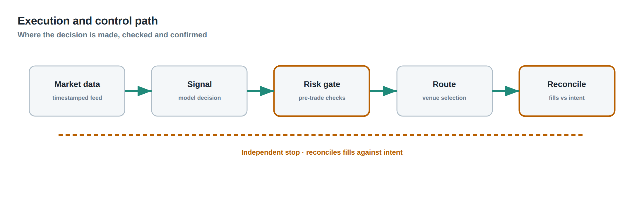
Stage 2 – Real‑time monitoring. A lightweight daemon subscribes to the equity feed of every strategy, updating the current peak and computing the live draw‑down. The daemon writes the draw‑down percentage and the elapsed time since the last peak to a shared memory segment that the execution engine reads every 100 ms. When a threshold is crossed, the daemon raises a flag in the risk‑control API.

Stage 3 – Automated response. The risk‑control API contains three callbacks: `on_warning`, `on_derisk`, and `on_shutdown`. Each callback is bound to a deterministic set of actions – logging, size scaling, order‑book flush – that execute without human approval. The callbacks also emit an audit event that includes the equity level, the threshold breached, and the timestamp, ensuring full traceability.

Stage 4 – Human oversight. While the automated actions protect the capital immediately, a risk analyst receives a real‑time alert on their dashboard. The analyst can inspect the underlying market data, verify that the trigger was not a false positive (e.g., a data‑feed glitch), and, if appropriate, adjust the subsequent thresholds for the remainder of the trading day. The analyst’s role is supervisory, not corrective, preserving the integrity of the pre‑defined ladder.

Stage 5 – Post‑mortem and re‑activation. After a shutdown, the strategy enters a “quarantine” state. A formal review is conducted, documenting the market conditions, execution anomalies, and model assumptions that failed. Only after the review committee signs off on a remediation plan – which may involve model retraining, latency upgrades, or revised risk parameters – does the strategy move back to the “ready” state, where it can be re‑enabled at a reduced risk level for a probationary period.

Controls that act before the damage

Preventative controls sit upstream of the draw‑down ladder and aim to reduce the probability that a breach occurs in the first place. One such control is the size‑capping rule, which limits the growth of position size to a function of recent realised volatility rather than a simple linear scaling. By tying size to volatility, the system automatically curtails exposure when market conditions become turbulent, thereby lowering the expected draw‑down.

Another pre‑emptive measure is execution‑quality monitoring. The platform continuously records fill rates, order‑to‑trade latency, and the frequency of stale orders. When the 99th‑percentile latency exceeds a pre‑set bound – for example 100 ms – the system temporarily routes orders through a higher‑quality gateway or reduces the order flow rate. This reduces the chance that an abnormal latency spike will generate a cascade of adverse selections that could trigger a draw‑down.

A third safeguard is the cross‑strategy correlation filter. Before each new trade, the system computes the marginal contribution to portfolio VaR, taking into account the current exposures of all strategies. If the marginal VaR of the proposed trade pushes the portfolio VaR beyond a defined ceiling, the trade is rejected or scaled down. By limiting the incremental risk, the filter prevents a single strategy from inadvertently dragging the whole portfolio into a draw‑down zone.

Finally, time‑under‑water limits are enforced as a proactive control. If a strategy remains more than 2 % below its recent peak for longer than a pre‑determined horizon – say 48 hours – the de‑risking callback is invoked even if the absolute loss is still within the warning band. This early‑stage de‑risking recognises that prolonged under‑performance often signals a shift in market regime rather than a transient blip.

How to measure whether it is working

Effectiveness is assessed by comparing the realised distribution of draw‑downs against the calibrated thresholds. A key metric is the breach frequency: the proportion of trading days in which any strategy exceeds its warning, de‑risking or shutdown band. In a well‑tuned system this frequency should be close to the statistical confidence level used during calibration – for instance 5 % for the warning band.

A second indicator is the recovery time after a de‑risking event. The average number of trading sessions required for equity to return to within 1 % of the pre‑draw‑down peak should decline over successive quarters, demonstrating that the reduced exposure is preserving optionality rather than merely postponing loss.

The size‑adjustment lag is also monitored. It measures the interval between a threshold breach and the execution of the corresponding size change. A lag of more than one execution cycle (typically 100 ms) is a red flag, suggesting that the monitoring daemon or the risk‑control API is a bottleneck. Reducing this lag directly improves the protective function of the ladder.

Lastly, the post‑mortem success rate – the fraction of shutdowns that result in a formal re‑activation after remediation – provides a proxy for the health of the overall risk culture. A high success rate indicates that shutdowns are being used as learning opportunities rather than punitive measures, reinforcing the discipline that the draw‑down controls are meant to instil.

The portfolio view

When draw‑down controls are applied at the strategy level, the portfolio‑wide impact can be visualised as a series of overlapping ladders. Each ladder contributes a piecewise‑linear reduction in aggregate risk exposure as the portfolio equity moves from its high water mark toward lower levels. The aggregate risk curve is therefore smoother than the sum of individual peaks, because de‑risking actions from multiple strategies often occur in the same market regime.

From a capital‑allocation perspective, the ladder framework creates a dynamic risk budget. As the portfolio experiences a draw‑down, the budget contracts automatically, freeing capital that can be redeployed to strategies that remain within their safe bands. This reallocation preserves overall Sharpe while protecting the desk from over‑leveraging a single under‑performing arm.

The portfolio view also highlights the importance of correlation monitoring. If two strategies exhibit a high positive correlation, a simultaneous breach of their warning bands can lead to a sharper portfolio‑level draw‑down than either would cause in isolation. By incorporating the correlation matrix into the threshold calibration, the desk can set tighter bands for highly correlated pairs, ensuring that the combined effect does not exceed the overall risk appetite.

In practice, the portfolio‑level draw‑down is reported daily alongside the individual strategy figures. The report includes the current peak, the deepest trough, the time‑under‑water, and the proportion of the risk budget currently active. This transparent snapshot allows senior management to see at a glance whether the desk is operating within its predefined risk envelope, and whether the ladder controls are delivering the intended protective effect.

—

Is your current draw‑down framework truly linked to automatic, evidence‑based actions, or does it merely record loss after the fact?

About the research behind this lesson

Andrew Lo's lectures build risk analysis from return distributions and statistical measures, rather than treating one realised result as a complete description of risk.

Applied to this lesson: For a fast strategy, median latency or average fill quality is not enough. The review has to include tail delays, stale-order frequency and the loss distribution when cancellation or routing behaves abnormally.

Two live systems, one desk

PULSE-X — power-packed HFT: high-frequency momentum on XAUUSD and EURUSD. System details · Live account

NIC-X — ultra-low drawdown: displaced-print arbitrage for large capital. System details · Live account

Start now: leave your email and request a free trial — we will send the pricing, the connection route and the trial terms. Pricing

Join the market discussion: Telegram @squawklive

Source: Risk and Return

Educational content only. Trading leveraged products involves risk.