November 8, 2026

What this problem really is

The intuitive notion that a profitable alpha can be scaled indefinitely is a myth that many junior traders discover the hard way. In a liquid electronic market every trade consumes a slice of the order‑book; the deeper the slice, the more the market price is nudged away from the pre‑trade mid. When a strategy is back‑tested with a modest notional – say a few hundred thousand dollars – the model may show a tidy Sharpe ratio, but the same algorithm run with a multi‑million‑dollar allocation can see its edge evaporate because the execution cost now exceeds the expected gross return.

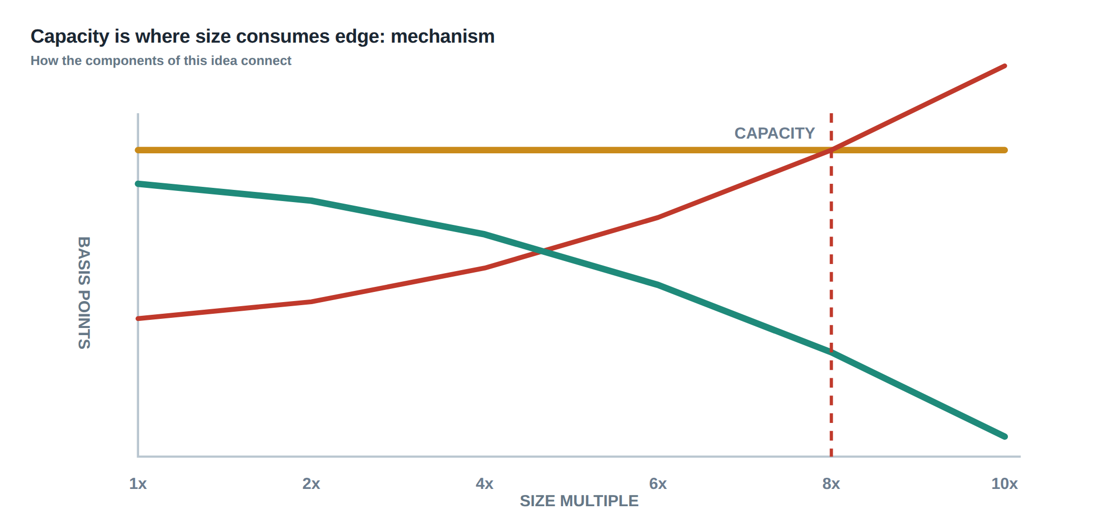
The root cause is capacity: the point at which the size of the order itself becomes a source of adverse price movement. Capacity is not a single static number; it is a curve that depends on the instrument’s average daily volume (ADV), the prevailing volatility, and the aggressiveness of the order. The curve is steep in thin sessions – for example, after the US market close or during macro‑event windows – and flatter when the order‑book is thick. When the curve is crossed, the net edge becomes zero or negative, and the strategy ceases to be viable.

The problem is compounded by the fact that many systematic traders treat execution cost as a fixed drag, often estimated from historical slippage. In reality the cost is a function of participation rate (the ratio of order size to market volume) and of the market’s instantaneous state. A static drag underestimates the true cost at the margin of capacity, leading to over‑allocation and unexpected draw‑downs.

How the mechanism works, step by step

Electronic markets operate as price‑time‑priority queues. When a limit order is submitted it joins a line at a particular price level; the order receives execution only when incoming marketable flow clears the queue ahead of it. The value of that queue position can be split into three components. First, the spread capture – the profit earned by buying at the bid and selling at the ask. Second, the adverse‑selection cost – the risk that the price moves against the order while it waits, eroding the spread. Third, the option value of staying in line – the expected benefit of retaining a place in the queue for a future price move.

If the order sits for a long time, the adverse‑selection component grows, and the option value may become negative. Conversely, a very aggressive order that crosses the spread immediately incurs a temporary impact cost: the market moves against the trader as the order eats through the best quotes. After the trade, a portion of that impact may persist as permanent impact, reflecting a new equilibrium price that incorporates the information revealed by the large trade.

The total cost therefore comprises spread loss, temporary impact, permanent impact and the opportunity cost of capital tied up while waiting for execution. All four terms are functions of participation rate and volatility. A higher participation rate raises both temporary impact (because more depth must be traversed) and permanent impact (because the market perceives a larger information signal). Higher volatility widens the spread but also increases the chance that a waiting order will be executed at a worse price.

A worked example with real numbers

Consider a mean‑reversion strategy on a high‑liquidity equity that trades a 10‑minute window around the market open. The instrument has an average daily volume of 20 million shares and a typical one‑minute volatility of 0.12 %. The model predicts a gross edge of 3 bps per trade, based on capturing half the average spread of 2 bps after accounting for a modest adverse‑selection estimate of 0.5 bps.

At a modest size of 10 000 shares (0.05 % of ADV, participation rate 0.5 % over the 10‑minute window) the temporary impact coefficient, calibrated from historical data, is 0.0004 bps per 0.1 % participation. The expected temporary impact is therefore 0.002 bps, negligible relative to the gross edge. Permanent impact is estimated at 0.001 bps per 0.1 % participation, adding another 0.001 bps. The total execution cost is roughly 0.003 bps, leaving a net edge of 2.997 bps – essentially the model’s prediction.

Now double the order to 20 000 shares, raising participation to 0.1 % of ADV per minute. Temporary impact scales non‑linearly: the coefficient rises to 0.0006 bps per 0.1 % participation because the order must walk down the book into less‑liquid price levels. The temporary impact now equals 0.006 bps. Permanent impact follows a similar non‑linear path, becoming 0.003 bps. The spread capture remains unchanged at 1 bps (half the spread), but the adverse‑selection component grows to 0.8 bps because the order sits longer while the market moves.

Summing the costs: spread loss 1 bps, adverse‑selection 0.8 bps, temporary impact 0.006 bps, permanent impact 0.003 bps, total cost 1.809 bps. The net edge drops to 1.191 bps – less than half the original. If the order were increased again to 40 000 shares, participation would reach 0.2 % per minute, temporary impact would climb to 0.015 bps, permanent impact to 0.008 bps, and adverse‑selection could exceed 1.2 bps as the queue position deteriorates. The net edge would then be negative, demonstrating that the cost more than doubles when size doubles.

The lesson is clear: scaling must be tested by incrementally increasing simulated size until the expected net edge reaches zero. The point at which this occurs defines the strategy’s capacity limit under the assumed market conditions.

Where it breaks in live markets

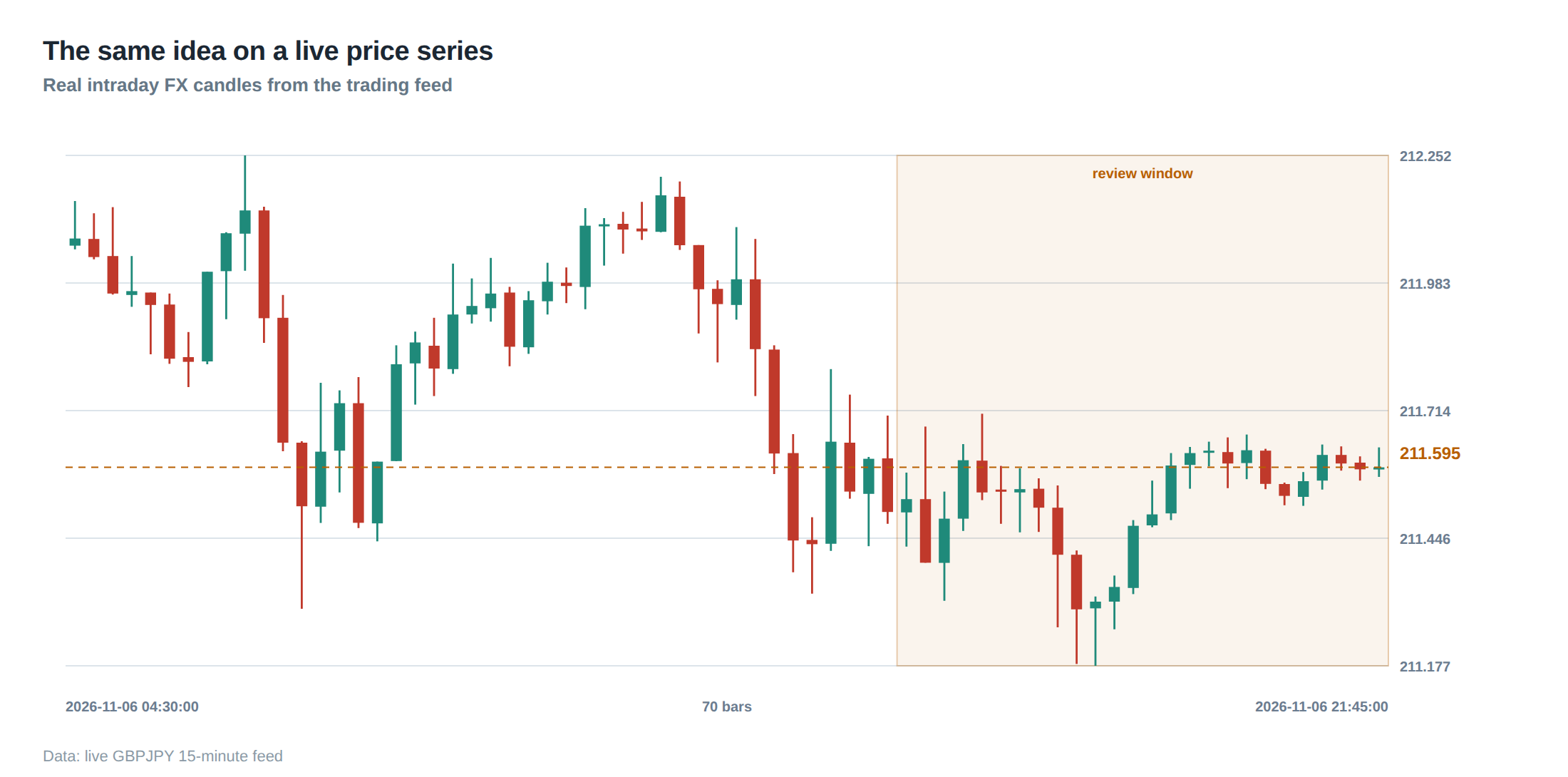
The theoretical capacity curve assumes a stationary market, yet real‑world trading encounters abrupt shifts. Thin sessions – for example, the first ten minutes after a major macro announcement – can see ADV collapse by 30 % while volatility spikes to 0.5 %. Participation rates that were previously safe now generate disproportionate temporary impact, and the permanent component can linger as the market re‑prices the new information.

Urgent exits amplify the problem. When a position must be liquidated within a few seconds – perhaps because a stop‑loss is triggered or a risk limit is breached – the trader cannot afford to wait for the queue to refill. The order becomes marketable, crossing the spread and forcing a large price concession. In such scenarios the opportunity cost of delayed execution becomes infinite; the only measurable cost is the realised slippage, which can be many times the normal impact estimate.

Another failure mode is hidden liquidity. Some venues allow iceberg orders that conceal depth; a strategy calibrated on displayed depth may underestimate the true cost of traversing the book. When a large order finally reveals hidden depth, the market can react sharply, turning what appeared to be a modest temporary impact into a permanent price shift.

The operating path, stage by stage

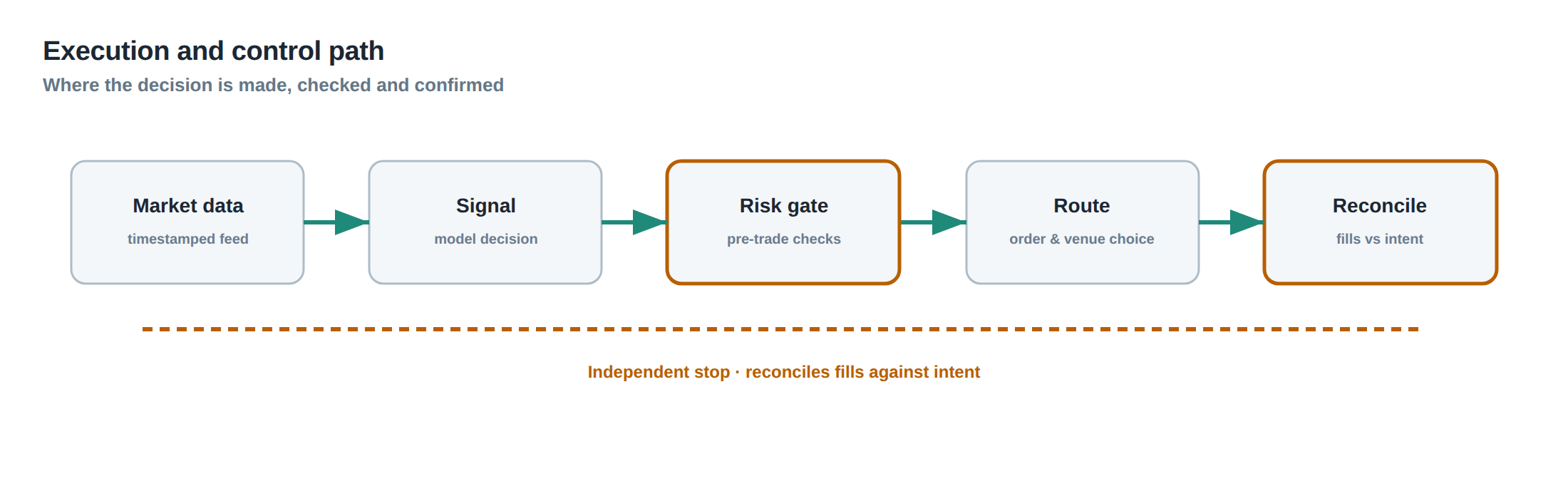
A robust capacity‑management workflow begins with a pre‑trade simulation. The algorithm is run on historical order‑book snapshots at varying notional levels, measuring the net edge after applying a realistic impact model that separates temporary and permanent components. The simulation continues until the edge curve flattens and eventually turns negative; the corresponding notional defines the provisional capacity limit.

The second stage is live monitoring. As the strategy runs, each execution is logged with timestamp, size, venue, realised price and the prevailing market depth. A sliding window aggregates these data to compute the realised participation rate and the realised slippage. The realised slippage is then plotted against the pre‑computed capacity curve.

If the realised slippage approaches the curve’s inflection point, the system triggers a scaling‑down signal. The signal can be a hard cap on notional, a reduction in order aggressiveness, or a shift to a less‑liquid venue where the impact model predicts a flatter curve. The final stage is post‑trade analysis, where the realised edge is compared to the forecasted edge. Discrepancies feed back into the impact model, refining the coefficients for temporary and permanent impact.

Controls that act before the damage

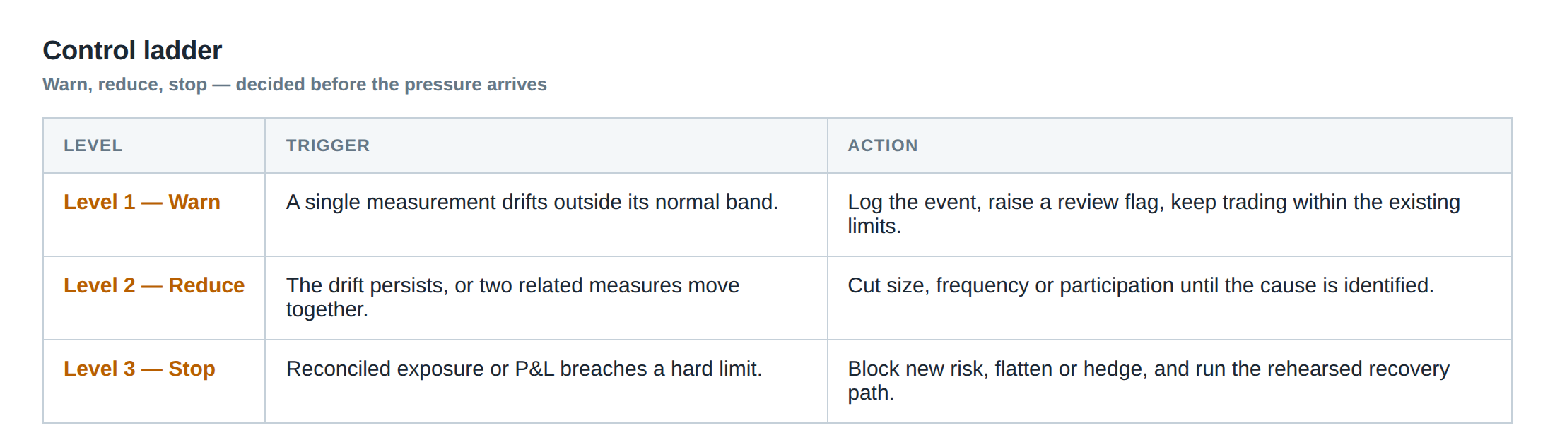
Preventive controls must be embedded both in the order‑routing logic and in the risk‑management layer. The first line of defence is a participation‑rate guard: before an order is sent, the system checks the projected participation against a dynamic threshold that tightens when volatility rises or when ADV drops below a pre‑set level.

A second guard is the “capacity ladder”. The ladder consists of discrete buckets of notional – for example, 0‑5 mm, 5‑10 mm, 10‑15 mm – each with an associated aggressiveness parameter. When the current notional crosses into a higher bucket, the algorithm automatically reduces the aggressiveness, perhaps by widening the limit price or by lengthening the time‑in‑force. This ensures that as size grows, the order’s footprint on the book does not increase proportionally.

A third safeguard is the “urgent‑exit throttle”. When a stop‑loss or margin call is triggered, the system first evaluates whether a partial, staggered liquidation would achieve the required risk reduction with less impact than an immediate market sweep. Only if the residual risk exceeds a pre‑defined tolerance does the system resort to a market‑order exit.

All three controls rely on real‑time market data feeds and on a low‑latency calculation of participation and volatility. They must be tested in a simulated environment that reproduces the latency and message‑drop characteristics of the production stack.

How to measure whether it is working

The primary metric is the realised net edge per trade, defined as the gross alpha minus the sum of spread loss, temporary impact, permanent impact and opportunity cost. This figure should be plotted over time alongside the expected net edge from the capacity model. A persistent gap indicates that the impact model is under‑estimating cost or that market conditions have shifted.

A secondary metric is the slippage‑to‑participation ratio. By regressing realised slippage against participation rate for each instrument, one can observe whether the slope has steepened, signalling a reduction in capacity. The regression should be performed on rolling windows of 1 hour to capture intra‑day dynamics.

The third diagnostic is the “capacity utilisation” ratio: realised notional divided by the pre‑computed capacity limit. When utilisation consistently exceeds 80 % the system should raise an alert, because the margin for error shrinks dramatically.

Finally, a “stress‑test” metric can be introduced by artificially inflating volatility in the impact model and observing how quickly the net edge collapses. If the model predicts a rapid loss of edge under modest volatility spikes, the live system should be configured to automatically reduce participation when volatility breaches the stress‑test threshold.

The portfolio view

Capacity is not a property of a single strategy in isolation; it is a constraint on the entire portfolio of signals. When multiple strategies target the same venue or the same underlying, their combined participation can push the market past the capacity curve even if each individual strategy remains within its own limit. Therefore, a portfolio‑level participation monitor is essential.

The monitor aggregates the projected participation of all active strategies in real time, weighting each by the liquidity of the instrument and by the current market depth. If the aggregate participation approaches a predefined portfolio‑wide threshold, the system can re‑allocate capital, throttling the most marginal strategies or shifting execution to alternative venues.

A further portfolio consideration is the correlation of execution costs across assets. During a market‑wide stress event, impact coefficients tend to rise together, turning a modest aggregate participation into a sizeable collective slippage. Modelling this correlation – for example, by estimating a common factor in the temporary‑impact regressions – enables the risk‑manager to set a more conservative portfolio capacity limit that accounts for systemic liquidity shocks.

By treating capacity as a shared resource, the desk can avoid the situation where a successful strategy silently erodes the edge of another, preserving the overall Sharpe ratio of the portfolio.

The discussion above has shown how a strategy that appears robust at modest size can be undone by its own orders, how to model and monitor the relevant cost components, and how to embed preventive controls at both the strategy and portfolio levels.

What steps will you take to embed a capacity‑aware feedback loop into your own execution workflow?

About the research behind this lesson

The seminar frames electronic markets as price-time-priority queues. It separates queue value into spread capture versus adverse-selection cost and the option value of retaining a place in line.

Applied to this lesson: An order lifetime therefore cannot be based on elapsed time alone: the system must reassess whether its queue position, expected spread and adverse-selection risk still justify keeping the order alive.

Two live systems, one desk

PULSE-X — power-packed HFT: high-frequency momentum on XAUUSD and EURUSD. System details · Live account

NIC-X — ultra-low drawdown: displaced-print arbitrage for large capital. System details · Live account

Start now: leave your email and request a free trial — we will send the pricing, the connection route and the trial terms. Pricing

Join the market discussion: Telegram @squawklive

Source: High-Frequency Trading and Modern Market Microstructure

Educational content only. Trading leveraged products involves risk.