October 28, 2026

What this problem really is

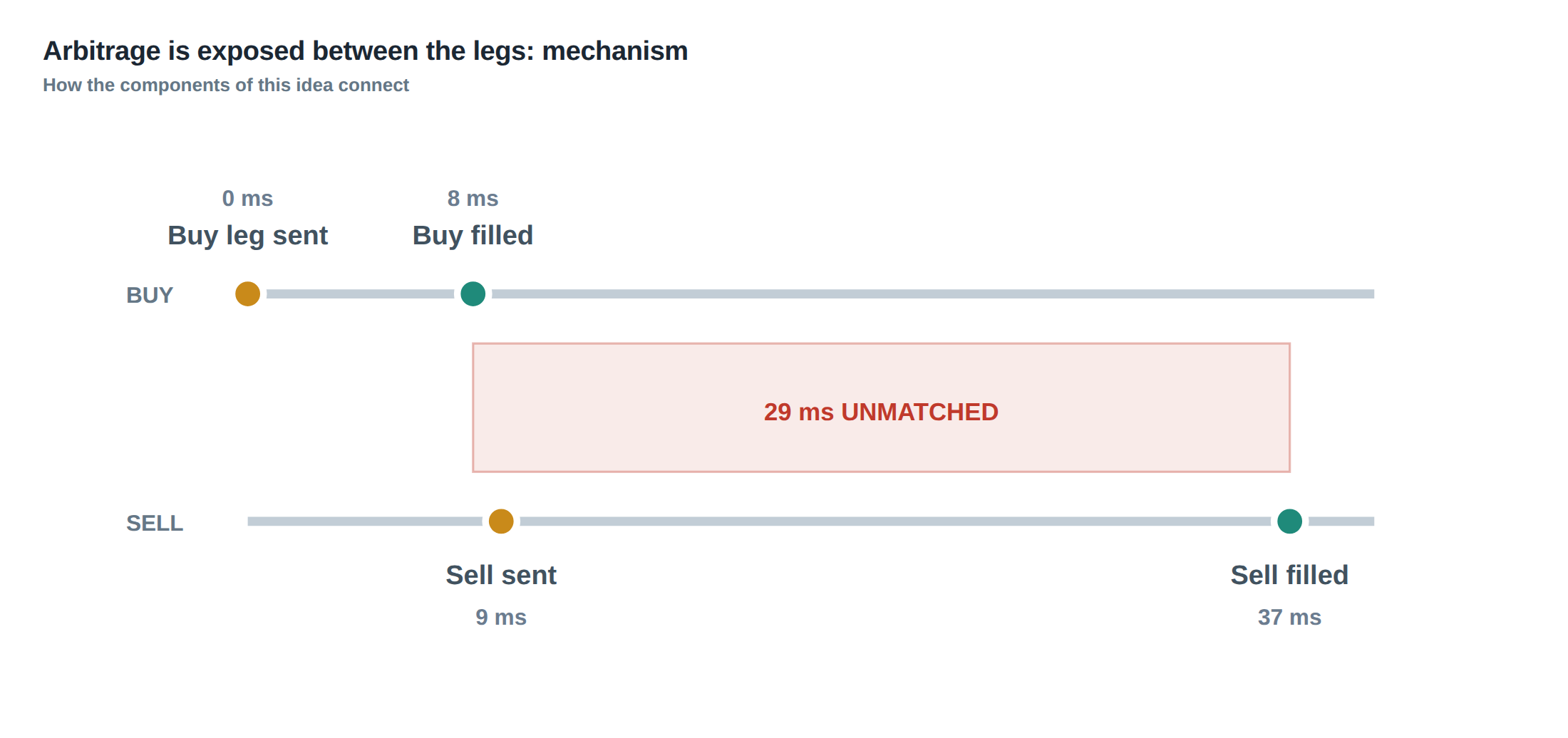
Arbitrage between two venues is often presented as a static spread that is market‑neutral by definition. In practice the spread only becomes neutral after the two legs have been executed, and the interval between the first fill and the second fill is a period of exposure. During that window the trader holds a directional position on the instrument that was filled first, while simultaneously bearing liquidity risk on the opposite side that is still pending. The risk is not merely theoretical; it is the difference between the price at which the first leg was taken and the price that will be required to unwind the unmatched leg when market conditions move against the intended arbitrage. The problem therefore is not the size of the spread but the dynamics of order execution across heterogeneous order books, each with its own minimum size, tick‑size, and queue discipline.

The literature on electronic markets models each limit order book as a price‑time‑priority queue. The value of a standing order can be decomposed into three components: the expected spread capture if the order is filled, the adverse‑selection cost that accrues while the order sits in the queue, and the option‑like value of retaining a place in line for a future price move. When a trader splits a strategy into two legs, the queue position of each leg evolves independently, and the overall exposure is the sum of the two queue values plus the cost of any imbalance that must be neutralised later.

Because the queue value is a function of both elapsed time and the evolving market state, a simple timer‑based order‑cancellation policy is insufficient. The system must continuously reassess whether the expected spread capture still outweighs the growing adverse‑selection risk and the cost of unwinding an unmatched leg. This continuous reassessment is the core operational challenge of “arbitrage exposed between the legs”.

How the mechanism works, step by step

The first step is to generate a synthetic spread by pairing a buy order on Venue A with a sell order on Venue B. Both orders are submitted simultaneously, each with a size that respects the venue‑specific minimum execution quantity. The order management system (OMS) records the target quantity for each leg and creates a real‑time ledger of filled versus remaining volume.

When an execution event arrives from either venue, the OMS updates the ledger, reduces the remaining quantity on that side, and recomputes the net exposure. If the fill is partial, the system calculates the residual exposure and checks it against pre‑defined hedge thresholds. If the remaining quantity on one side exceeds the hedge threshold, the OMS may decide to place an additional order on the same venue (a “reroute”) or to cancel the outstanding order and replace it with a marketable order to neutralise the imbalance.

A cancel threshold is also defined: if the expected time to completion, derived from recent fill‑rate statistics, exceeds a certain percentile of the completion‑time distribution, the system may abort the pending leg and instead execute a hedge in the opposite direction on the same venue. The decision logic therefore hinges on three quantitative inputs: the current filled‑vs‑remaining ratio, the venue‑specific minimum size constraint, and the statistical model of completion times.

Throughout the life of the spread the OMS must also monitor the cost of neutralising the unmatched leg. This cost is the sum of the spread that would be lost by executing a market order at the current best price and any slippage caused by the market impact of the hedge. If that cost breaches a predefined “unmatched‑leg cost” threshold, the system will pre‑emptively unwind the filled leg, even if the opposite leg has not yet been filled, to avoid a larger loss later.

A worked example with real numbers

Consider a trader who wishes to exploit a $0.08 spread between two equities: a bid of 100.12 on Venue A and an ask of 100.20 on Venue B. The target arbitrage size is 10 000 shares. Venue A imposes a minimum order size of 2 000 shares, while Venue B requires a minimum of 1 500 shares. The OMS therefore submits a 10 000‑share buy limit order at 100.12 to Venue A and a 10 000‑share sell limit order at 100.20 to Venue B, both with a time‑in‑force of 5 seconds.

Within 300 ms the buy order on Venue A receives a partial fill of 4 000 shares at 100.12. The ledger now shows 4 000 filled on the buy side and 0 on the sell side, leaving 6 000 shares to be bought and 10 000 shares to be sold. The OMS consults its completion‑time model, which indicates that, historically, Venue B fills 70 % of orders of this size within 1 second, but the remaining 30 % take up to 4 seconds. The hedge threshold is set at a remaining‑quantity ratio of 0.6; because the sell side still has 10 000 shares unfilled (a ratio of 1.0), the system does not yet trigger a hedge.

At 1 200 ms the sell order on Venue B receives a fill of 3 500 shares at 100.20. The exposure now consists of a long position of 4 000 shares and a short position of 3 500 shares, leaving a net long of 500 shares. The remaining quantities are 6 000 to buy and 6 500 to sell. The OMS recalculates the expected cost of neutralising the 500‑share imbalance. The current best bid on Venue A is 100.13 and the best ask on Venue B is 100.19, implying a cost of 0.06 per share to unwind, i.e. $30. The unmatched‑leg cost threshold is $50, so the system tolerates the imbalance for now.

At 2 800 ms the buy side receives an additional fill of 5 000 shares, completing the buy leg (total 9 000 shares filled). The sell side still has 6 500 shares outstanding. The net exposure is now a short of 6 500 – 9 000 = 2 500 shares. The OMS sees that the remaining sell quantity exceeds the hedge threshold (2 500 / 10 000 = 0.25 < 0.6) and that the projected completion time for the remaining sell leg, based on the last 1 500‑share fill rate, is now estimated at 3 seconds, which breaches the cancel threshold of 2 seconds. Consequently, the system cancels the remaining sell order on Venue B and immediately places a market sell for 2 500 shares on Venue A at the prevailing bid of 100.13. The cost of this forced hedge is 2 500 × 0.01 = $25, well below the $50 limit, but the trader has now turned an apparent risk‑free spread into a realised position that incurred a $25 slippage cost and a $30 cost from the earlier imbalance, totalling $55 of execution drag.

The example demonstrates that the interval between fills can convert a theoretical arbitrage into a directional exposure that must be managed actively, and that the cost of neutralising the unmatched leg can exceed the spread if the system’s thresholds are not calibrated to the venue‑specific fill dynamics.

Where it breaks in live markets

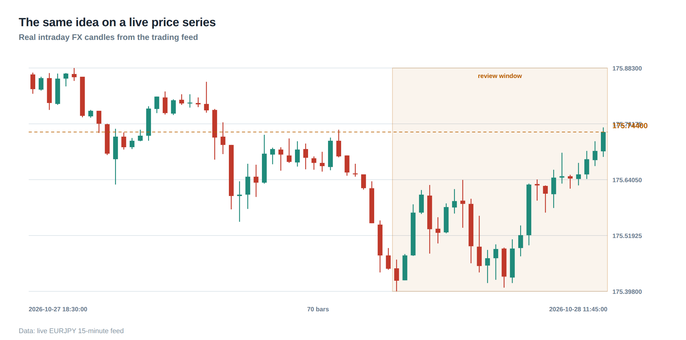
In a live environment the assumptions that underpin the completion‑time model are constantly violated. Market depth can evaporate in milliseconds, causing the fill rate to drop dramatically. Venue‑specific minimum sizes can become binding when the order book thins, forcing the OMS to split the intended quantity into multiple smaller orders that each suffer higher adverse‑selection risk.

Latency differentials between the two venues exacerbate the problem. If Venue A is co‑located and Venue B is accessed via a longer network path, the first leg will typically fill earlier, leaving the second leg exposed for a longer period. In periods of heightened volatility, the best bid‑ask spread can widen beyond the expected $0.08, turning the intended capture into a loss if the unmatched leg must be executed at a worse price.

Another failure mode is the “queue‑jump” phenomenon. When a large order is placed on a venue, other participants may respond by cancelling and re‑submitting at a more aggressive price, effectively leap‑frogging the original order. The adverse‑selection cost therefore spikes, and the expected spread capture erodes. If the OMS relies only on elapsed time to trigger cancellation, it will miss this rapid deterioration.

Finally, regulatory constraints such as minimum resting times or order‑to‑trade ratios can prevent the system from instantly rerouting or cancelling orders, leaving the trader with an unhedged exposure that may be amplified by market moves.

The operating path, stage by stage

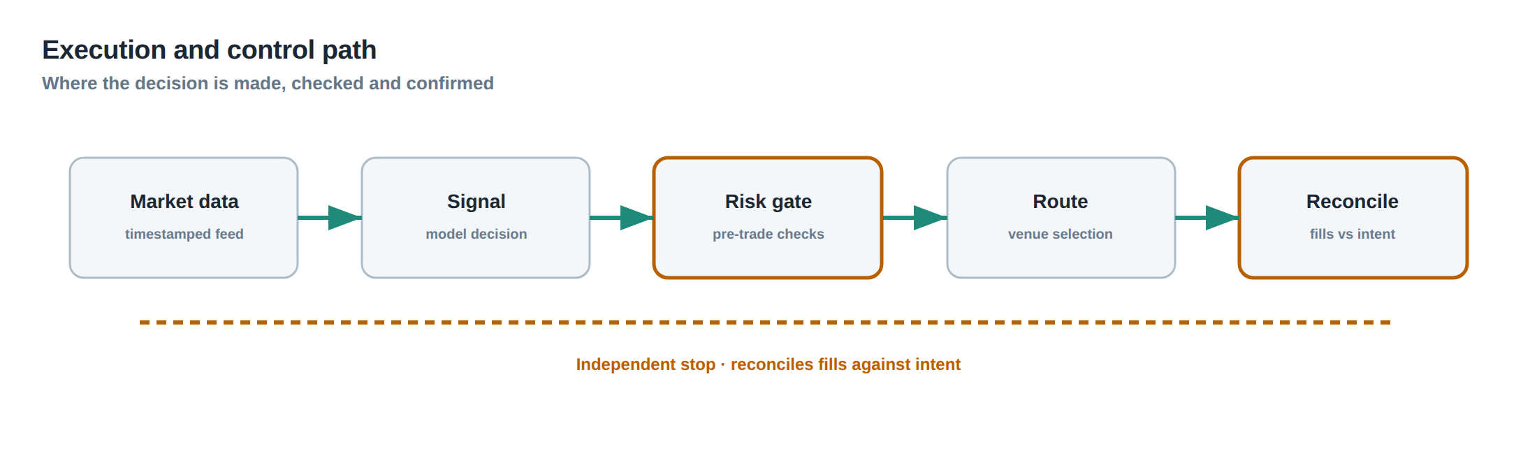
The first stage is the generation of the synthetic spread, where the algorithm selects the two venues, determines the optimal size respecting each venue’s minimum, and creates the paired orders. The second stage is the monitoring loop, which ingests execution reports, updates the filled‑vs‑remaining ledger, and recomputes exposure metrics after every event.

The third stage is the decision engine, which evaluates the hedge, cancel, and reroute thresholds. If the remaining quantity on one side falls below the hedge threshold, the engine may submit an additional order on the same venue or on a third venue with better liquidity. If the projected completion time exceeds the cancel threshold, the engine sends a cancellation request for the pending leg.

The fourth stage is the execution of the neutralisation trade. When a decision to hedge is taken, the system calculates the market impact and slippage cost of the required marketable order, compares it to the unmatched‑leg cost threshold, and then routes the order to the venue offering the best price‑size combination.

The final stage is the post‑trade reconciliation, where the system records the realised spread capture, the cost of any forced hedge, and the latency statistics for each leg. These data feed back into the statistical model that predicts completion times, allowing the thresholds to be adjusted dynamically.

Controls that act before the damage

A robust control framework places safeguards at each stage of the operating path. Before order submission, a pre‑trade validator checks that the requested size satisfies the minimum‑size constraints of both venues and that the combined spread exceeds the sum of the estimated adverse‑selection cost and a safety margin.

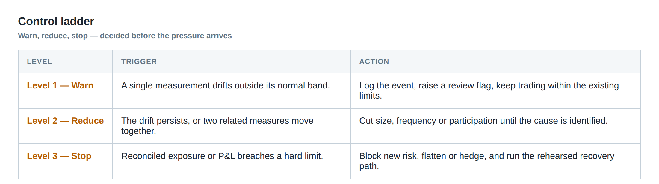
During the monitoring loop, a real‑time exposure limiter tracks the net directional position. If the net long or short exceeds a configurable percentage of the total intended spread, an automatic hedge is triggered regardless of the completion‑time estimate.

The decision engine is equipped with a dynamic threshold manager that adjusts hedge and cancel thresholds based on recent fill‑rate volatility. When volatility spikes, the manager tightens the cancel threshold, prompting earlier cancellations to avoid prolonged exposure.

A final pre‑execution check verifies the current market depth on the venue where a hedge would be placed. If the depth is insufficient to absorb the required size without moving the price beyond the acceptable slippage, the system either fragments the hedge into smaller slices or aborts the entire spread, logging the event for post‑mortem analysis.

Together these controls aim to intervene before the exposure becomes material, reducing the probability that an apparent arbitrage degenerates into an outright directional position.

How to measure whether it is working

Effectiveness is measured by three complementary metrics. The first is the realised spread capture per attempted arbitrage, calculated as the gross spread minus the sum of all execution costs, including slippage, market impact, and any forced‑hedge expenses. The second is the distribution of completion times for each leg, expressed as percentiles; a shift of the 90th percentile to longer durations indicates deteriorating execution quality.

The third metric is the frequency and magnitude of unmatched‑leg hedges. By aggregating the cost of all forced hedges over a rolling window, the desk can assess whether the thresholds are set appropriately. A rising trend suggests that the hedge threshold is too permissive or that market conditions have changed.

Statistical process control charts can be employed to monitor these metrics in real time, flagging out‑of‑control points that require immediate investigation. The post‑trade reconciliation data also feed into machine‑learning models that refine the completion‑time forecasts, thereby tightening the decision engine’s parameters.

The portfolio view

From a portfolio perspective, each spread is a micro‑position that contributes to the overall market‑neutral exposure of the desk. The net directional exposure of all open spreads should remain close to zero, otherwise the desk inherits systematic risk that defeats the purpose of arbitrage trading.

Aggregating the realised spread capture across the portfolio provides a signal of the desk’s edge after accounting for execution drag. If the aggregate capture consistently falls below the expected theoretical spread, it may indicate that the queue‑value model is mis‑specified or that the venue‑specific thresholds are too lax.

Conversely, a high incidence of forced hedges that erode the spread capture can be mitigated by rebalancing the portfolio towards venues with faster fill rates or by adjusting the size of each spread to stay within the sweet spot of the venue’s liquidity curve. The portfolio view therefore informs both strategic allocation of capital across venues and tactical parameter tuning of the OMS.

In summary, the apparent neutrality of a spread is an illusion that disappears the moment one leg is filled and the other remains pending. By continuously tracking filled quantities, modelling completion‑time distributions, and enforcing disciplined hedge and cancel thresholds, a prop‑trading desk can manage the directional and liquidity risk that resides in the interval between fills.

What steps will you take to ensure that the interval between legs does not turn a theoretical arbitrage into an unintended market exposure?

About the research behind this lesson

The seminar frames electronic markets as price-time-priority queues. It separates queue value into spread capture versus adverse-selection cost and the option value of retaining a place in line.

Applied to this lesson: An order lifetime therefore cannot be based on elapsed time alone: the system must reassess whether its queue position, expected spread and adverse-selection risk still justify keeping the order alive.

Two live systems, one desk

PULSE-X — power-packed HFT: high-frequency momentum on XAUUSD and EURUSD. System details · Live account

NIC-X — ultra-low drawdown: displaced-print arbitrage for large capital. System details · Live account

Start now: leave your email and request a free trial — we will send the pricing, the connection route and the trial terms. Pricing

Live chat and updates: Telegram @xtrskhft

Source: High-Frequency Trading and Modern Market Microstructure

Educational content only. Trading leveraged products involves risk.