October 5, 2026

What this problem really is

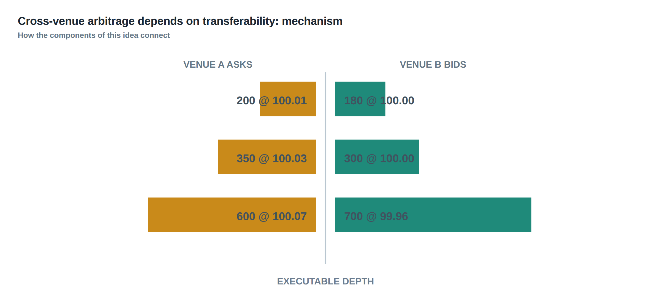
The temptation to treat any two quoted prices as a ready‑made arbitrage is a classic mistake on modern multi‑venue desks. A price on Venue A and a price on Venue B may appear to diverge by several ticks, but the divergence is only exploitable if the two legs can be executed, settled and cleared under the exact same capital and inventory constraints. In practice the limiting factor is transferability – the ability to move the required quantity of the instrument, or the cash that backs it, from one venue to the other fast enough to complete the round‑trip before the price gap erodes.

Transferability is governed by three intertwined layers: the order‑book depth that is actually executable, the fee‑rebate schedule that changes the net spread, and the settlement or withdrawal rules that dictate when the proceeds of the first leg become available for the second. When any of these layers is mis‑aligned, the apparent spread collapses into a paper illusion. The problem therefore sits at the intersection of market microstructure, operational logistics and capital management, rather than purely at the level of price feeds.

A further nuance is that the “best‑bid / best‑ask” snapshot hides the queue position of any pending order. If a trader places a limit order at the top of the book on Venue A, the order may sit behind a sizeable queue of higher‑priority participants. The realised execution price can be several ticks worse than the displayed quote, especially when the queue is long or when the order is large relative to the displayed depth. The same applies on the opposite side of the arbitrage. Consequently, the true arbitrage opportunity is the difference between the executable depth on both sides after accounting for all frictions.

How the mechanism works, step by step

The first step is to acquire a real‑time view of executable depth on each venue. This requires a market‑data subscription that provides not only the top‑of‑book but also the size available at each price level for the next few ticks. The algorithm then calculates the gross spread that would be earned if both legs were filled at those levels, ignoring fees and settlement timing.

Next, the system adds the venue‑specific fee schedule. Exchange fees are typically charged on the maker side, while rebates are paid to takers. If the arbitrage involves taking liquidity on one side and providing it on the other, the net fee can swing the spread by a full tick or more. The calculation therefore subtracts the taker fee on the buying leg and adds the maker rebate on the selling leg (or vice‑versa), yielding a net spread.

The third step evaluates the transferability of the capital or inventory required for the second leg. If the arbitrage is a cash‑and‑carry type, the cash received from the first execution must be withdrawable or transferable to the second venue within the expected latency. If the arbitrage is inventory‑based, the physical or electronic holdings must be available on the destination venue, which may involve settlement cycles, clearing‑house lock‑up periods or internal transfer queues. The algorithm therefore imposes a transfer cost – either a fixed fee for a cross‑venue transfer or an opportunity cost equal to the market risk borne while the funds are in transit.

Only after these three adjustments does the system decide whether the residual spread exceeds a pre‑defined profitability threshold. If it does, the order is sent to the venue with the best execution probability; otherwise the opportunity is discarded as non‑executable.

A worked example with real numbers

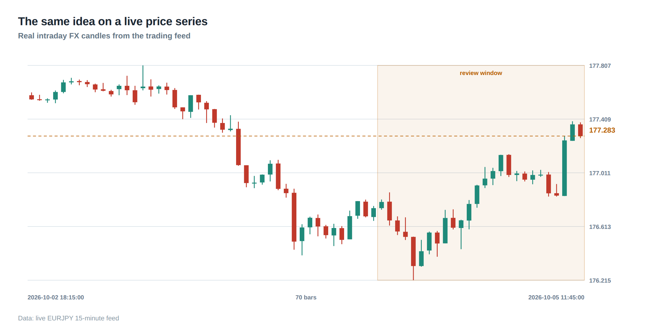
Consider a futures contract on an equity index that trades on Venue X and Venue Y. At 09:45 GMT the best‑bid on X is 3 500.00 with 12 contracts available, and the best‑ask on Y is 3 500.25 with 8 contracts available. The raw spread is therefore 0.25 points, or 25 ticks if the contract tick size is 0.01. A naïve view would label this a 25‑tick arbitrage.

Venue X charges a taker fee of 0.4 % of notional and offers a maker rebate of 0.2 %. Venue Y charges a taker fee of 0.3 % and a maker rebate of 0.1 %. The arbitrage plan is to buy on X (taking liquidity) and sell on Y (providing liquidity). The notional per contract is 10 USD, so buying 8 contracts on X costs 8 × 3 500.00 × 10 = 280 000 USD. The taker fee on X is 0.004 × 280 000 = 1 120 USD. Selling 8 contracts on Y yields 8 × 3 500.25 × 10 = 280 020 USD, and the maker rebate on Y is 0.001 × 280 020 ≈ 280 USD. The net cash flow before transfer costs is therefore:

Revenue = 280 020 – 280 = 279 740 USD Cost = 280 000 + 1 120 = 281 120 USD Net = ‑1 380 USD, a loss of 13.8 USD per contract.

Even before considering transfer latency, the arbitrage is unprofitable because the fee differential outweighs the 0.25‑point price gap. Suppose the desk holds the required 8 contracts on Venue Y already, eliminating the need to transfer inventory. The transfer cost is then zero, but the net loss remains. If instead the desk had the cash on X and needed to move it to Y, the internal transfer takes 250 ms and incurs a fixed cost of 30 USD per transfer. Adding that pushes the loss to 1 410 USD.

Now imagine the same price gap appears but the depth on X is only 4 contracts while Y still offers 8. The executable gross spread falls to 4 × 25 = 100 ticks, or 1 000 USD of gross profit. After fees and the 30 USD transfer charge, the net becomes a modest 40 USD gain, well within the desk’s noise floor. The example shows how a seemingly large quoted gap can evaporate once fees, depth and transferability are accounted for, or conversely how a smaller gap can become viable when inventory is pre‑positioned.

Where it breaks in live markets

In live trading the most common failure mode is the assumption that the quoted depth will remain static long enough to execute both legs. In reality, order flow on high‑frequency venues can consume the displayed depth within a few milliseconds. If the algorithm sends the first leg and the second leg is delayed by network latency, the opposite side may have moved, leaving the trader with an unfilled order or a worse price than anticipated.

A second break point is the settlement‑cycle mismatch. Some venues settle on a T+0 basis for cash, while others require a T+2 clearing for the same instrument. When the arbitrage relies on the proceeds of the first leg to fund the second, the cash may be locked in a settlement queue, forcing the trader to use pre‑allocated capital that could have been deployed elsewhere. The opportunity therefore disappears unless the desk maintains a buffer of capital on the destination venue.

Third, fee structures can change intra‑day. Many exchanges adjust maker‑rebate rates in response to volatility spikes, and some introduce temporary taker‑fee surcharges during market stress. An algorithm that does not refresh the fee schedule in real time may continue to flag opportunities that are no longer profitable after the fee shift.

Finally, venue outages and connectivity glitches are rare but catastrophic. If the primary venue suffers a micro‑second outage while the algorithm is waiting for the second leg, the first leg may be filled but the second leg never arrives, leaving the desk with an unwanted inventory position and exposure to market moves. The risk is amplified when the arbitrage is leveraged, as the margin requirement can be breached instantly.

The operating path, stage by stage

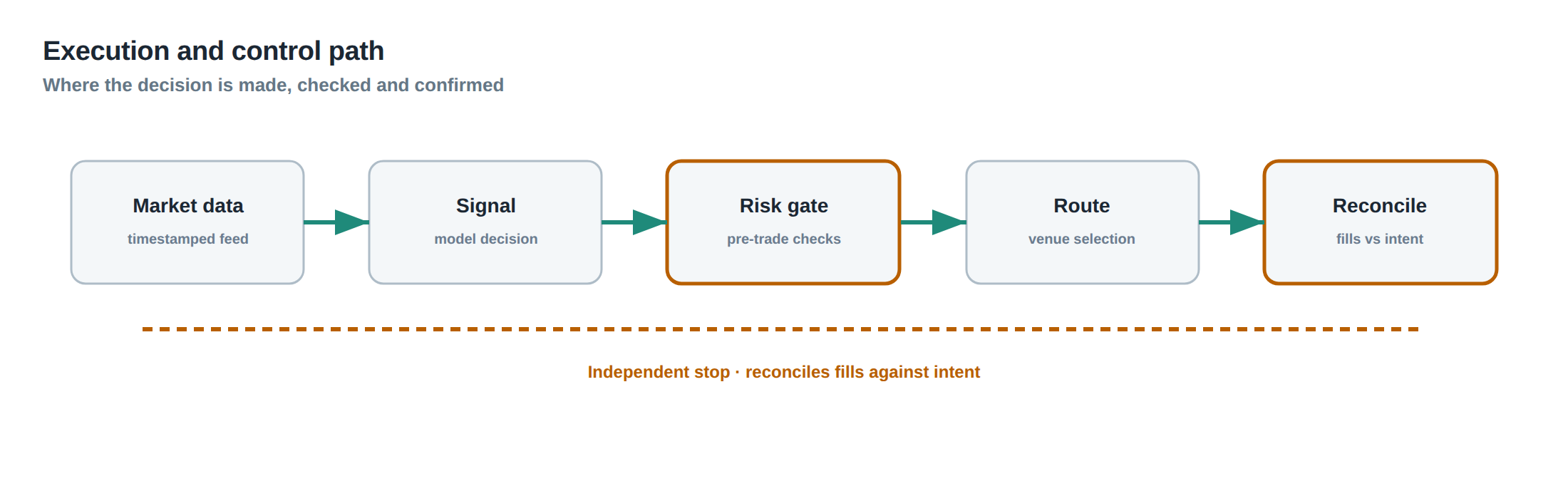
Stage 1 – Market‑data ingestion: The system subscribes to depth‑of‑book feeds from all relevant venues, normalises timestamps to a common clock and stores the last N price levels for each side. The data pipeline must guarantee sub‑millisecond latency to preserve the integrity of the depth snapshot.

Stage 2 – Opportunity detection: A sliding window evaluates the executable spread across venues, applying the current fee schedule and a static transfer‑cost estimate. The output is a list of candidate legs with the required size, expected execution price and a profitability score.

Stage 3 – Pre‑trade validation: Before any order is emitted, the engine checks inventory balances, available cash, and the status of any pending internal transfers. If the required inventory is not already on the destination venue, the system either initiates a pre‑positioning transfer or discards the candidate.

Stage 4 – Order routing: The algorithm selects the venue with the highest probability of immediate fill, based on historical fill‑rate models, and submits a limit order at the price that matches the executable depth. The order is tagged with a short time‑to‑live (TTL) to avoid lingering in the queue.

Stage 5 – Post‑execution reconciliation: Once the first leg reports a fill, the system updates the inventory ledger, triggers the transfer of cash or contracts if needed, and immediately sends the second‑leg order. If the second leg fails, a cancellation or hedge is automatically generated.

Stage 6 – Feedback loop: Execution statistics (fill ratio, slippage, fee realised) are fed back into the detection model, allowing the profitability threshold to be dynamically adjusted in line with observed market conditions.

Controls that act before the damage

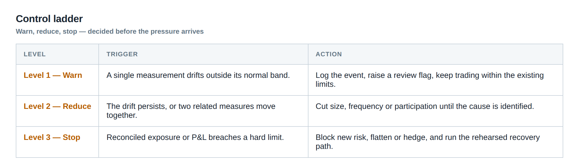
A robust pre‑trade control suite must enforce that no arbitrage order is launched unless the net spread after fees, transfer costs and expected slippage exceeds a safety margin, typically set at two to three times the standard deviation of recent execution noise. This margin guards against transient spikes in the quoted spread that are not supported by depth.

Inventory limits are another essential control. The desk should maintain a minimum buffer of the instrument on each venue equal to the maximum size of any single arbitrage leg observed over the past hour. If the buffer falls below the threshold, the system blocks further arbitrage attempts until the buffer is replenished through a scheduled transfer.

Transfer‑risk limits cap the amount of cash that can be tied up in transit. For venues with known settlement latency, the system calculates the maximum exposure that can be safely held while waiting for funds to clear, and rejects any arbitrage that would exceed this exposure.

Finally, a real‑time health monitor watches connectivity to each venue, latency spikes, and fee‑schedule broadcasts. If any metric deviates beyond preset bounds, the arbitrage module is automatically disabled, preventing the submission of orders under degraded conditions.

How to measure whether it is working

Performance measurement starts with the gross realised spread: the difference between the execution price of the buy leg and the sell leg, multiplied by the contract size and the number of contracts filled. From this figure the system subtracts the actual fees paid, the maker rebates received, and any explicit transfer fees incurred. The resulting net spread is the true profit per trade.

A second metric is execution efficiency, defined as the ratio of the filled quantity to the displayed executable depth at the time of order entry. Values below 70 % indicate that the algorithm is frequently over‑estimating depth, signalling a need to tighten the depth filter.

The capital utilisation ratio measures how much of the pre‑positioned inventory or cash buffer is actually employed in profitable arbitrage versus sitting idle. High utilisation suggests that the buffer size is appropriate; low utilisation may indicate excess capital that could be redeployed elsewhere.

Risk‑adjusted performance is captured by the Sharpe‑type statistic that divides the average net spread per trade by the standard deviation of net spreads over a rolling window. A declining ratio often precedes a regime shift, such as a fee schedule change or a market‑structure alteration, prompting a review of the underlying assumptions.

The portfolio view

From a portfolio perspective, cross‑venue arbitrage is a micro‑layer that sits beneath the primary directional exposure. The net P&L from arbitrage should be uncorrelated with the market beta of the underlying instrument, providing a modest diversification benefit. However, the operational risk – especially the risk of being stuck with an unwanted inventory after a failed second leg – introduces a short‑term exposure that must be hedged.

The desk can hedge this exposure by maintaining a dynamic delta hedge on the same instrument in a separate, low‑latency venue. If the arbitrage leg on Venue Y fails, the hedge can be adjusted within a few milliseconds to neutralise the resulting directional risk. The cost of this hedge is the spread on the hedging venue, which must be factored into the overall profitability calculation.

Liquidity risk is another portfolio consideration. Large arbitrage positions can consume a non‑trivial fraction of the displayed depth, thereby moving the market against the desk’s own orders. The optimal position size is therefore a function of both the available depth and the market impact model, which should be calibrated on a per‑instrument basis.

Finally, the aggregate capital allocated to arbitrage should be capped as a proportion of the desk’s total risk budget. Since arbitrage profits are typically thin, the desk must ensure that the capital tied up in pre‑positioned inventory or in transit does not erode the capacity to take larger, higher‑conviction bets. Regular stress‑testing of the arbitrage engine against extreme latency spikes and venue outages helps maintain this balance.

Do you have a systematic way to verify that the inventory you hold on each venue truly matches the size of the arbitrage opportunities you are chasing?

About the research behind this lesson

The seminar frames electronic markets as price-time-priority queues. It separates queue value into spread capture versus adverse-selection cost and the option value of retaining a place in line.

Applied to this lesson: An order lifetime therefore cannot be based on elapsed time alone: the system must reassess whether its queue position, expected spread and adverse-selection risk still justify keeping the order alive.

Explore PULSE: System details

PULSE live account: Verify the live account on FX Blue

Live chat and updates: Telegram @xtrskhft

Source: High-Frequency Trading and Modern Market Microstructure

Educational content only. Trading leveraged products involves risk.