October 16, 2026

What this problem really is

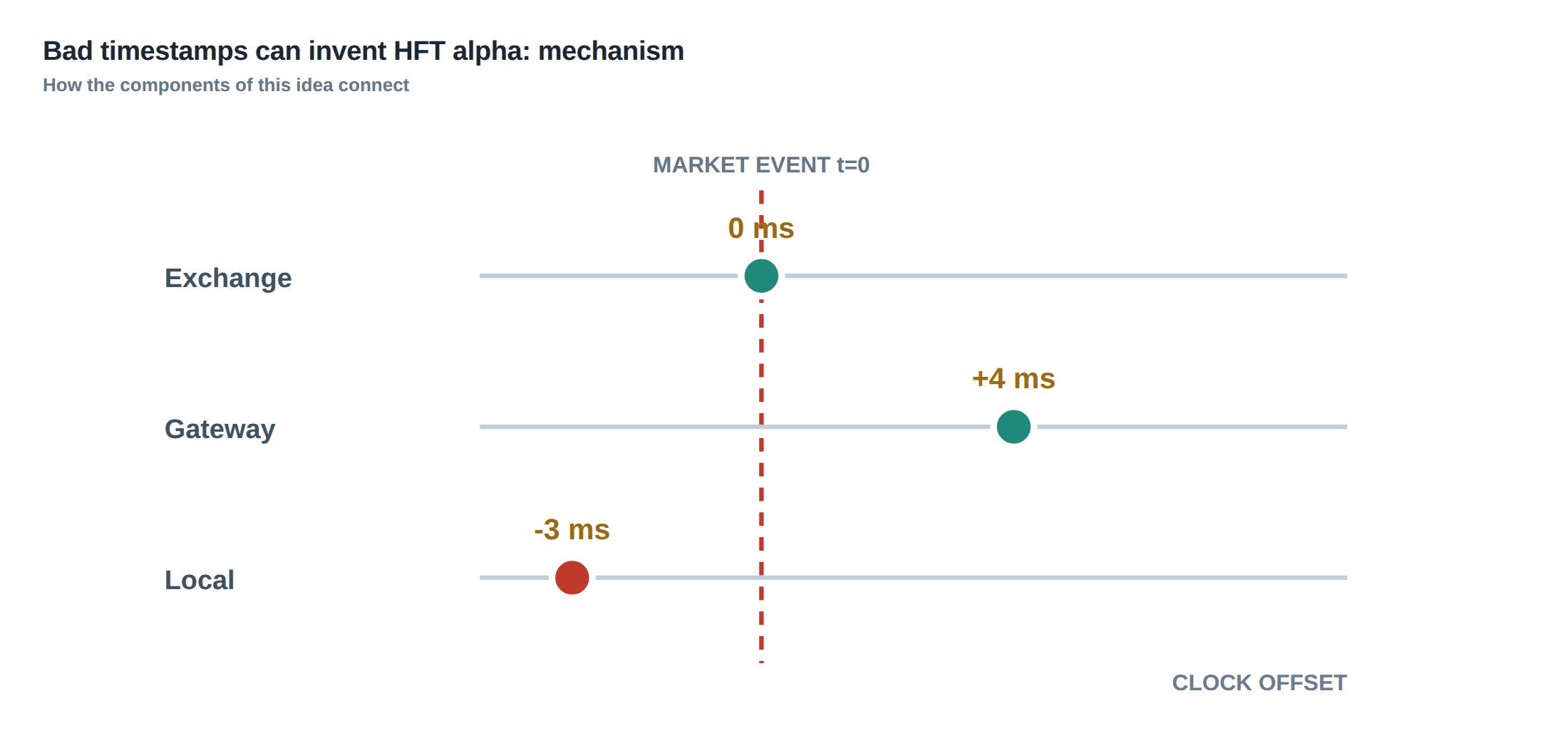
High‑frequency trading relies on the assumption that the clock attached to every event – a market data packet, an order‑submission, a fill – is a faithful representation of the instant the event became known to the algorithm. In practice the timestamps that arrive from an exchange, from a gateway, and those generated by a local NIC are produced by different time‑bases. The exchange may use a GPS‑derived clock, the gateway a NTP‑synchronised server, and the local machine a CPU‑based timer that drifts under load. When these clocks are not perfectly aligned, the microsecond‑level ordering of events becomes ambiguous. A strategy that appears to act on a quote before a trade actually executed may be exploiting a phantom lead that never existed in real time. The illusion of “alpha” is therefore a by‑product of mis‑aligned timestamps rather than a genuine predictive edge.

The problem is compounded by the fact that most back‑testing pipelines simply concatenate timestamps from disparate sources and treat them as a single timeline. The resulting data set can contain out‑of‑order packets, duplicate messages, or correction frames that overwrite earlier values. If the analysis does not explicitly preserve the original sequence numbers and the provenance of each timestamp, the reconstructed market view is internally inconsistent. Consequently, any statistical inference drawn from such a view inherits the timing error.

In a professional prop‑trading environment, where execution latency is measured in single‑digit microseconds, even a 10‑µs offset between the exchange timestamp and the local receipt time can shift a trade from being “before” a price move to “after” it. The core thesis is that microsecond‑level analysis is unreliable unless the three timestamp domains – exchange, gateway, and local – are stored separately, monitored for drift, and reconciled against a trustworthy reference clock. Only then can we separate genuine signal from artefact.

How the mechanism works, step by step

First, the exchange stamps every market data packet with its own clock, typically derived from a disciplined GPS source. The packet then traverses a proprietary gateway where a second timestamp is attached, reflecting the moment the gateway forwards the packet to the client. Finally, the client’s NIC records the time at which the packet is placed into the receive buffer, using the host’s high‑resolution timer. These three timestamps travel together, but most vendors strip the intermediate values, leaving only the exchange time or the local receipt time.

Second, the client must maintain a continuous measurement of the offset between its local clock and the exchange clock. This is achieved by periodically comparing the exchange timestamp embedded in a known reference message (for example, a heartbeat) with the local receipt time, then applying a low‑pass filter to estimate drift. The estimated offset is stored alongside each event, allowing the reconstruction of a “common‑time” view where every event can be placed on the exchange’s timeline with a quantified uncertainty.

Third, the data pipeline must preserve the original sequence numbers supplied by the exchange and any correction or retransmission messages that follow. When a correction arrives, the system replaces the stale entry but also records the correction timestamp and the reason code. By doing so, the pipeline can later test for out‑of‑order arrivals and duplicate events, and can flag periods where the feed reliability deteriorates. Only after these steps are completed can the analyst safely compute latency statistics, such as median fill time, tail latency, and the probability of a stale order reaching the market.

A worked example with real numbers

Consider a back‑test of a simple spread‑arbitrage strategy that monitors the EUR/USD spot price and the corresponding futures contract. At 09:30:00.123456 UTC the exchange publishes a trade message for the futures at 1.1050, stamped with the exchange clock (T_ex = 09:30:00.123456). The gateway forwards the packet and adds its own timestamp (T_gw = 09:30:00.123470). The local NIC receives the packet at T_loc = 09:30:00.123520.

Two milliseconds later, at 09:30:00.125500 UTC, the exchange sends a quote update for the spot market indicating a price move to 1.1048, with T_ex = 09:30:00.125500, T_gw = 09:30:00.125515, and T_loc = 09:30:00.125560. In the raw data set that only retains the local timestamps, the trade appears at 09:30:00.123520 and the quote at 09:30:00.125560, preserving the correct order. However, if the gateway clock were 20 µs ahead of the exchange clock, the quote’s exchange timestamp would be 09:30:00.125480, and after applying the offset the reconstructed common‑time would place the quote at 09:30:00.125460, still after the trade.

Now imagine a subtle bug: the data ingestion layer mistakenly discards the gateway timestamp and records the exchange timestamp as the local receipt time. The trade would be logged at 09:30:00.123456, the quote at 09:30:00.125500, and the strategy would correctly infer that the trade preceded the quote. But if the exchange’s clock were 30 µs slow relative to the gateway, the true order would be reversed – the quote arrived first, but the back‑test would show the opposite. The back‑test would then report a positive P&L for every occurrence of this pattern, inventing alpha that vanishes in live trading because the strategy is actually reacting to stale information.

The lesson is that without preserving the three timestamps, monitoring offset, and applying the correction, the back‑test can appear to predict a price change when, in reality, the trade feed is timestamped earlier than the quote update that actually arrived first. The numerical discrepancy may be as small as 20‑30 µs, yet over thousands of trades it translates into a statistically significant illusion of profitability.

Where it breaks in live markets

In a live deployment, the mis‑alignment manifests as a sudden increase in order‑rejection rates and a higher proportion of “stale‑order” fills. When the exchange’s internal clock drifts because of GPS signal loss, the timestamps attached to market data become inconsistent with the gateway’s forwarding time. The client, unaware of the drift, continues to assume that a received trade is contemporaneous with the latest quote, and submits an order based on an outdated view of the order book. Execution venues then reject the order or fill it at a price that no longer reflects the intended arbitrage.

The problem is amplified during periods of high network congestion, where packet re‑ordering becomes common. A quote that should have arrived first may be delayed behind a trade due to queuing in the router. If the system does not retain the original sequence numbers, it cannot detect that the trade was processed out of order. Consequently, the latency histogram shows a deceptively low median latency, while the tail – the critical region for HFT – contains a non‑negligible mass of events that were effectively “late”.

Another failure mode occurs when the exchange issues correction messages to amend earlier trade timestamps. If the back‑testing engine discards these corrections, the reconstructed market history retains the original, erroneous timestamps. The live system, however, receives the corrected timestamps and must adjust its internal state. The mismatch between the historical model and the live feed leads to a systematic bias in the strategy’s expectation of fill quality, causing the realised P&L to diverge sharply from the back‑tested projection.

The operating path, stage by stage

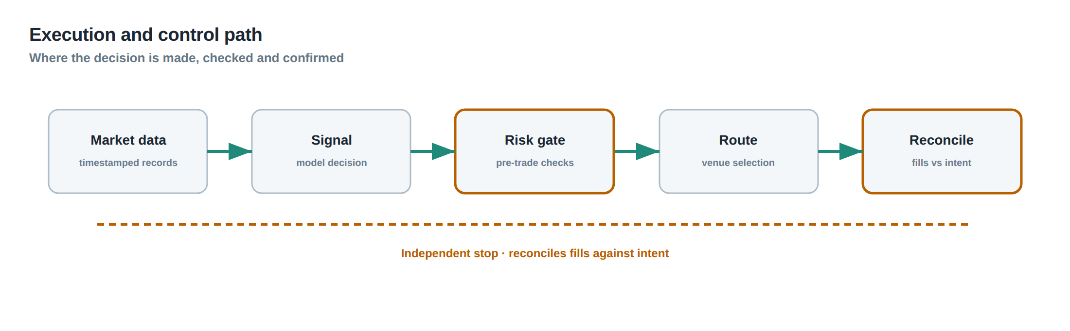
Stage one begins at the exchange gateway, where every inbound packet is tagged with a high‑resolution gateway timestamp and the original exchange timestamp. The gateway also emits a periodic heartbeat that includes both timestamps, providing the raw material for offset estimation. Stage two is the network interface on the client machine; the NIC records the time at which each packet is placed into the receive queue, using the host’s monotonic clock. The driver then forwards the packet, together with all three timestamps, to the market‑data handler.

Stage three is the ingestion service, which writes the raw packet to a time‑series store, preserving the exchange, gateway, and local timestamps in separate fields. It also logs the sequence number and any correction flags. Stage four is the latency‑normalisation engine, which continuously computes the offset between the local and exchange clocks by comparing heartbeat timestamps, applies a smoothing filter, and stores the resulting offset curve. Stage five is the reconstruction module, which uses the offset curve to map every event onto a common exchange timeline, annotating each event with an uncertainty band that reflects the measured jitter. Finally, stage six is the strategy core, which consumes the normalised stream, makes decisions, and records its own timestamps for order submission and receipt, completing the loop for later performance analysis.

Each stage must be instrumented independently, because a failure in any one can corrupt the entire chain. For instance, if the NIC driver mis‑reports timestamps due to a kernel bug, the downstream normalisation will propagate the error, and the strategy will be built on a flawed view of causality. By isolating the stages and storing their outputs separately, the desk can audit the provenance of any timing anomaly and pinpoint the source of the discrepancy.

Controls that act before the damage

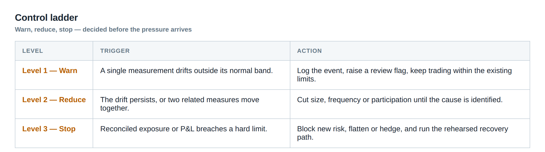
The first line of defence is a clock‑synchronisation watchdog that raises an alarm whenever the estimated offset exceeds a pre‑defined threshold, for example 15 µs. The watchdog monitors the heartbeat‑derived offset in real time and, upon breach, can automatically pause order submission or switch to a fallback data feed that provides a verified timestamp source.

A second control is the sequence‑number validator, which checks that incoming packets arrive in strict monotonic order per instrument. When a gap or a duplicate is detected, the validator flags the event and triggers a correction‑request to the exchange, ensuring that the data store contains the most recent, authoritative version of the market state.

A third safeguard is the “stale‑order detector”, which compares the time of the latest quote (after normalisation) with the time an order is generated. If the gap exceeds the strategy’s latency budget, the order is either delayed until a newer quote arrives or cancelled outright. This prevents the algorithm from acting on information that, due to clock drift, is already obsolete.

These controls are implemented as separate services that run in parallel to the main strategy engine, so that a failure in one does not cascade to the others. By enforcing strict bounds on clock offset, sequence integrity, and data freshness before any order leaves the desk, the probability of generating phantom alpha is dramatically reduced.

How to measure whether it is working

Measurement begins with the distribution of the offset between the local clock and the exchange clock. The desk should maintain a rolling window of the offset’s mean, standard deviation, and the 99.9th‑percentile value. A stable system will show a mean near zero and a 99.9th‑percentile below the pre‑set alarm threshold.

Next, the latency histogram of the normalised events must be examined. The median latency is useful, but the tail – especially the 99.99th percentile – is the critical metric for HFT. If the tail exceeds the strategy’s maximum tolerable latency, the system is not delivering reliable timing information, regardless of how low the median appears.

Finally, the back‑test versus live‑test divergence is a practical indicator. By running the same strategy on a data set that includes the three‑timestamp reconstruction and on a live feed that uses the same pipeline, the desk can compute the difference in realised P&L, win‑rate, and drawdown. A negligible difference suggests that the timing controls are effective; a systematic bias points to residual mis‑alignment or unhandled correction messages. Regular reporting of these metrics, together with automated alerts when thresholds are breached, provides continuous assurance that the timing infrastructure is functioning as intended.

The portfolio view

When the timing infrastructure is sound, the portfolio’s risk profile reflects genuine market risk rather than artefacts of mis‑timed data. The return distribution of a microsecond‑scale strategy will exhibit a thin centre and fat tails only if the underlying market dynamics generate such behaviour, not because the back‑test has inadvertently shifted events forward in time. Consequently, the portfolio’s risk metrics – value‑at‑risk, expected shortfall, and tail‑loss probability – become meaningful inputs for capital allocation and stress testing.

Conversely, if timestamps are unreliable, the portfolio may appear to have a superior Sharpe ratio driven by phantom alpha. The apparent reduction in tail risk is illusory; once the strategy is deployed live, the true latency distribution surfaces, and the portfolio suffers unexpected drawdowns. By integrating the timestamp‑validation pipeline with the risk‑management system, the desk can enforce limits on median latency, tail latency, and stale‑order frequency as part of the overall risk budget. This alignment ensures that the quantitative models, the execution engine, and the capital allocation framework all operate on a consistent, trustworthy chronology of market events.

In practice, the desk should treat the timing infrastructure as a first‑order risk factor, on a par with market volatility or liquidity. Its health is monitored daily, its limits are codified in the same way as position limits, and any breach triggers the same escalation procedures as a breach of market risk thresholds. By doing so, the desk safeguards against the most insidious source of spurious alpha – the illusion created by bad timestamps.

Do you have a systematic process in place to audit the alignment of exchange, gateway, and local timestamps before you trust any microsecond‑level signal?

About the research behind this lesson

Andrew Lo's lectures build risk analysis from return distributions and statistical measures, rather than treating one realised result as a complete description of risk.

Applied to this lesson: For a fast strategy, median latency or average fill quality is not enough. The review has to include tail delays, stale-order frequency and the loss distribution when cancellation or routing behaves abnormally.

Explore PULSE: System details

PULSE live account: Verify the live account on FX Blue

Live chat and updates: Telegram @xtrskhft

Source: Risk and Return

Educational content only. Trading leveraged products involves risk.