October 27, 2026

⛶

What this problem really is

Direct Market Access (DMA) is often equated with “the fastest route to the exchange”. In practice the fastest network path does not guarantee the best execution price. Modern electronic venues operate as price‑time‑priority queues; an order that arrives first may still sit behind a deep queue of resting orders, incur a large spread, or be exposed to adverse‑selection risk. The execution quality therefore depends on three interacting layers: the physical latency of the connection, the micro‑structure of the venue (queue depth, order‑type rules, matching engine latency), and the available liquidity at the moment the order is inserted.

When a trader submits a decision price – the price at which the algorithm decides to trade – the order first meets a benchmark arrival price (the market price observed at the moment the order is sent) and later a final fill price (the price at which the trade actually settles). The difference between these three points is the true cost of routing. If the routing logic simply selects the venue with the shortest round‑trip time, it may repeatedly place orders into a venue where the queue length forces the order to wait for several milliseconds, during which the market can move against the trader. In contrast, a slightly slower network path that lands on a venue with shallow depth and tighter spreads can deliver a better net price.

The problem is therefore not a binary “direct = good” decision but a continuous optimisation problem that must be measured, monitored and re‑optimised in real time. Without systematic measurement, a desk may be blind to systematic leakage caused by sub‑optimal routing choices.

How the mechanism works, step by step

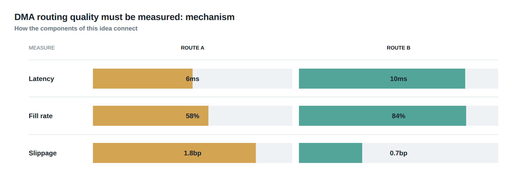
The first step is the generation of a decision price by the strategy engine. This price is derived from the algorithm’s signal, risk limits and the prevailing market snapshot. The decision price is then handed to the order router, which evaluates a set of pre‑defined routing rules – latency, venue fee structure, historical fill rates, and queue‑depth forecasts.

If the router selects a venue, the order is transmitted over the DMA link. The exchange acknowledges receipt with a timestamped “order accepted” message; this marks the arrival price. At this point the order joins the venue’s limit‑order book at the best price level that satisfies the price‑time priority rules. The order’s position in the queue is a function of the number of resting orders ahead, their sizes, and any hidden or iceberg orders that may not be visible to the router.

The matching engine continuously scans the queue for incoming marketable orders. When a counter‑party arrives, the engine executes against the earliest resting order at that price level, reducing the queue depth. If the order is fully filled, the final fill price is recorded; if only a partial fill occurs, the order remains in the queue until either it is completely filled, cancelled, or expires.

Should the router detect that the order’s expected time‑to‑fill exceeds a pre‑set threshold, it may issue a cancellation and reroute the residual quantity to an alternative venue. The cancellation outcome – whether the order was successfully withdrawn before a fill, or partially filled before the cancel – must be logged for later analysis.

A worked example with real numbers

Consider a mid‑day EUR/USD liquidity‑seeking order for 1 million units. The algorithm’s decision price is 1.1025. The router evaluates two venues: Venue A, reachable via a 30 µs network path, and Venue B, reachable via a 45 µs path. At the moment of routing, Venue A shows a best‑bid of 1.1024 with a queue depth of 800 k at that price, while Venue B shows a best‑bid of 1.1025 with a queue depth of 150 k.

The router selects Venue A because of the lower latency. The order is transmitted and the exchange acknowledges receipt at 1.1024 – the arrival price. Because the queue depth is 800 k, the order sits behind 800 k of resting volume. Within the next 5 ms, the market moves up to 1.1026, and a large market sell order consumes the 800 k at 1.1024, then matches the first 200 k of our order at 1.1025. The order is partially filled for 200 k at 1.1025, and the remaining 800 k remains in the queue.

The router’s timeout is set at 8 ms. After 8 ms the order is still unfilled, so a cancellation request is sent. The exchange confirms cancellation of the remaining 800 k after 2 ms, but during that window another market buy order arrives at 1.1026 and executes against the residual 800 k, delivering a fill at a worse price. The final fill price for the whole order is therefore a weighted average of 1.1025 for the first 200 k and 1.1026 for the remaining 800 k, giving an overall execution price of 1.10258.

If the router had chosen Venue B, the order would have arrived at 1.1025, faced a queue of only 150 k, and been fully filled within 3 ms at the decision price. The overall execution price would have been 1.1025, a 0.8 pip improvement over the Venue A outcome despite the longer network latency.

Where it breaks in live markets

In live trading the assumptions that underpin routing decisions are constantly violated. Queue depth can change in a few microseconds as hidden orders surface, and market participants may deliberately place large “liquidity‑taking” orders to clear queues and force slower venues to lose order flow. Moreover, venue‑specific rules – such as minimum order size, hidden order priority, or post‑trade reporting delays – can introduce hidden latency that is invisible to the router’s latency‑only model.

A common failure mode is the “sticky queue” effect. An order that repeatedly lands on the same venue after a cancellation may retain a lower priority position because the exchange treats the re‑submission as a new order at the back of the line. If the router does not reset its internal queue‑depth estimate after each cancellation, it will continue to underestimate the true time‑to‑fill.

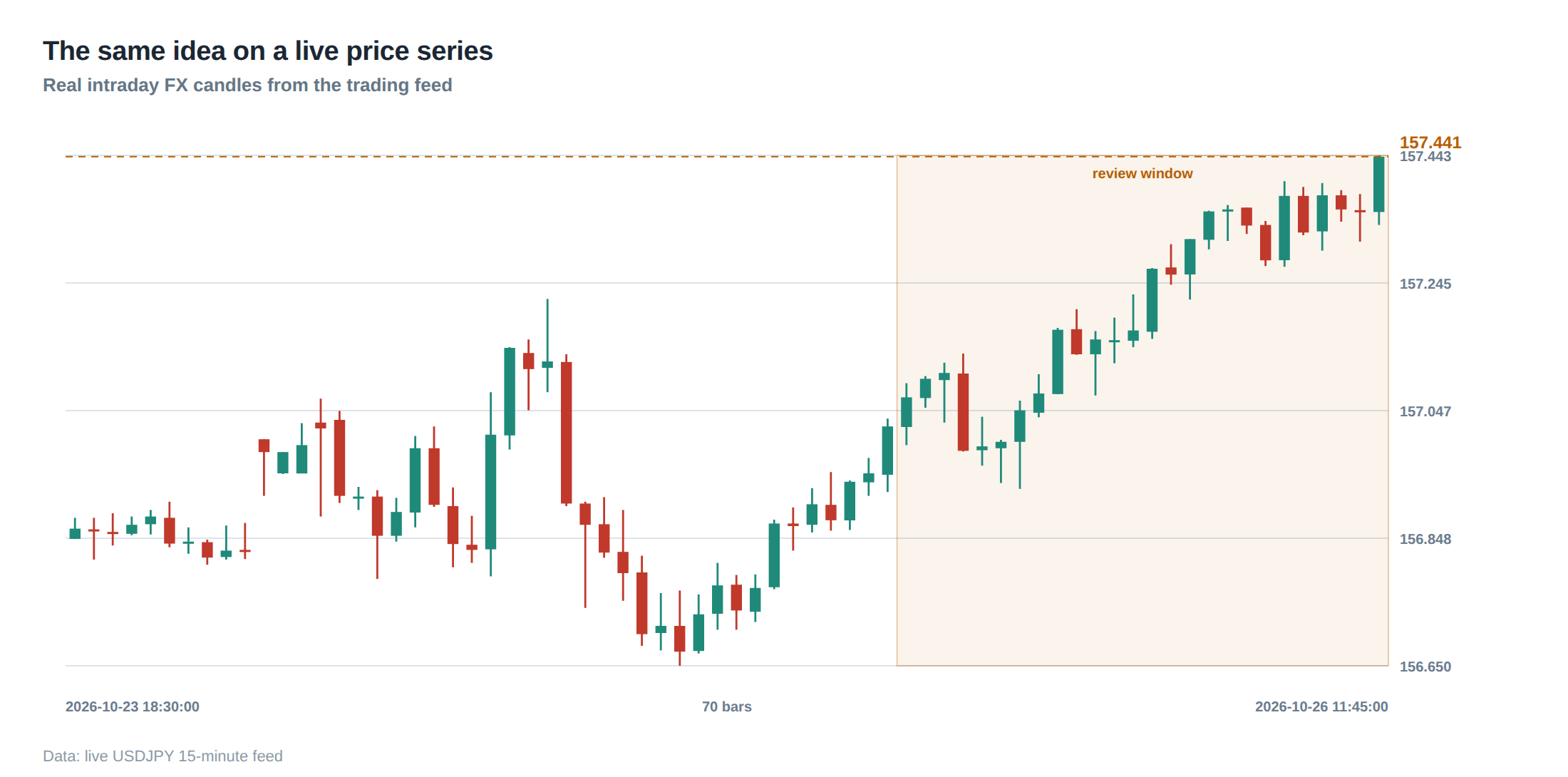
Another breakdown occurs when the market experiences rapid price swings. The decision price may become stale within the round‑trip time, especially in high‑frequency environments. If the router does not incorporate a real‑time price‑watchdog that aborts the order before it reaches the exchange, the order may be filled at a price far worse than the original signal, inflating slippage and adverse‑selection costs.

Finally, the interaction between multiple algorithmic strategies on the same venue can create “self‑cannibalisation”. One strategy’s aggressive order can fill the queue that another strategy’s order is waiting on, effectively turning the venue into a source of internal market impact. Without cross‑strategy visibility, the router cannot anticipate this feedback loop.

The operating path, stage by stage

The first stage is the signal capture and decision‑price generation, where the strategy translates market data into a target price and size. The second stage is the routing decision, which consults a rule‑engine that weighs latency, historical fill probability, and venue‑specific cost components. The third stage is the transmission over the DMA link, where the order is serialized, encrypted, and sent to the exchange’s gateway.

The fourth stage is the exchange acknowledgement, which returns a timestamped receipt and places the order in the venue’s order book. At this point the order’s queue position is known only indirectly, through depth‑of‑book snapshots and estimated execution probability. The fifth stage is the monitoring loop, where the router continuously evaluates fill progress, market movement, and elapsed time against the pre‑set thresholds.

If the thresholds are breached, the sixth stage is the cancellation request, which must be sent with sufficient headroom to be honoured before the next fill. The seventh stage is the re‑routing decision, where the residual quantity is re‑evaluated against the venue matrix and possibly sent to an alternative venue. The final stage is the post‑trade reconciliation, where the actual fill price, time‑to‑completion, and any partial fills are logged against the decision and arrival prices for performance analysis.

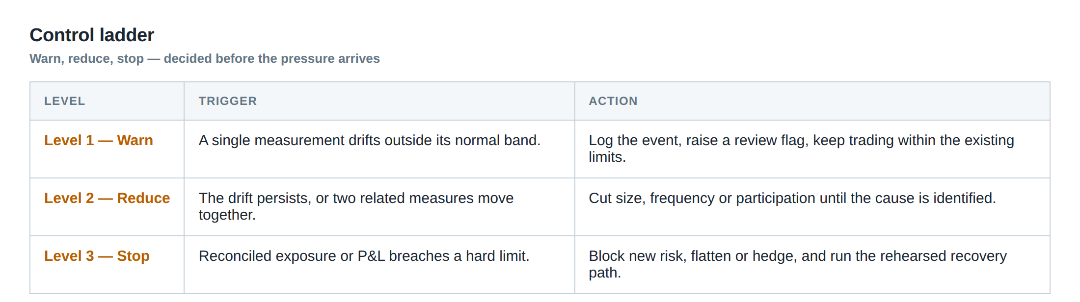
Controls that act before the damage

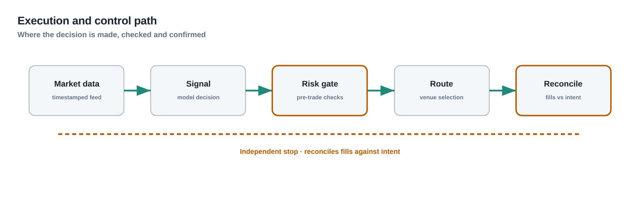
A robust control framework begins with pre‑trade validation. The order must be checked against venue‑specific constraints such as minimum tick size, order‑type compatibility, and maximum allowable size. This prevents immediate rejections that would waste latency.

Next, a dynamic queue‑depth estimator is required. By ingesting real‑time depth‑of‑book updates and historic fill‑rate curves, the estimator can predict the expected time‑to‑fill for each venue. When the predicted time exceeds the algorithm’s maximum acceptable latency, the estimator flags the venue as unsuitable for the current order.

A third control is the “price‑watchdog”. As soon as the market price moves more than a predefined tolerance from the decision price, the watchdog triggers an early cancellation, thereby avoiding fills at adverse prices. The watchdog can be configured per‑instrument to reflect volatility regimes.

Finally, a “routing‑logic audit” runs in parallel to the live router. It records every routing decision, the data that fed the decision, and the outcome of the order (filled, partially filled, cancelled). By periodically replaying these logs against a reference model, the desk can detect drift in the router’s behaviour, such as an increasing reliance on a single venue that no longer offers the best queue characteristics.

How to measure whether it is working

Measurement begins with the three‑point price benchmark: decision price, arrival price, and final fill price. The spread between decision and arrival captures pure latency cost, while the spread between arrival and final fill captures queue‑related slippage and adverse‑selection cost. By aggregating these spreads across a large sample of orders, the desk can compute an average execution cost per venue.

Partial‑fill analysis adds another dimension. For each order, the proportion of volume filled at each price level is recorded, together with the time taken to achieve each fill. The metric “time‑to‑completion” – the interval from arrival to the moment the order is fully executed or cancelled – is then compared against the router’s internal timeout thresholds. A systematic excess of time‑to‑completion indicates that the queue‑depth estimator is under‑estimating waiting times.

Cancellation outcome is also critical. A “clean cancel” – where no execution occurs after the cancel request – is the ideal, whereas a “partial cancel” where some volume is filled after the request signals a race condition that may be mitigated by extending the cancel‑lead time.

Finally, the impact on market depth must be measured. By monitoring the venue’s depth‑of‑book before and after order insertion, the desk can assess whether the routing decision caused a measurable price move (market impact). If the same decision price repeatedly results in a larger impact on a particular venue, the routing logic should downgrade that venue for similar future orders.

The portfolio view

When the execution quality of a single venue is examined in isolation, the picture may appear satisfactory. However, a portfolio‑wide view reveals cross‑venue interactions that can erode overall performance. For example, if a large proportion of the desk’s flow is routed to Venue A, the venue may respond by widening its spread or increasing queue depth, thereby degrading the quality of subsequent orders.

Conversely, diversifying across venues can smooth the impact of temporary congestion. By allocating a fraction of the order flow to a secondary venue with higher latency but lower queue depth, the desk can capture the spread advantage while limiting the exposure to any single venue’s micro‑structure risk. This “routing diversification” must be quantified by measuring the marginal cost of each additional venue against the incremental reduction in queue‑related slippage.

The portfolio view also incorporates the cost of cancellations and re‑routing. Each cancel incurs exchange fees and may generate a small market impact as the order disappears from the book. Summing these costs across all orders provides a “routing‑efficiency ratio” – the proportion of total execution cost that is attributable to routing decisions rather than market movement. Optimising this ratio is the ultimate objective of any DMA quality‑measurement programme.

In practice, the desk should maintain a rolling dashboard that displays the three‑point price spread, average time‑to‑completion, partial‑fill ratios, and routing‑efficiency ratio for each venue and for the aggregate portfolio. By setting target thresholds for each metric, the desk can trigger automatic adjustments to the routing rule‑engine before performance deteriorates.

Do you currently monitor the full three‑point price chain and queue‑depth forecasts, or are you still relying solely on latency as the proxy for execution quality?

About the research behind this lesson

The seminar frames electronic markets as price-time-priority queues. It separates queue value into spread capture versus adverse-selection cost and the option value of retaining a place in line.

Applied to this lesson: An order lifetime therefore cannot be based on elapsed time alone: the system must reassess whether its queue position, expected spread and adverse-selection risk still justify keeping the order alive.

Two live systems, one desk

PULSE-X — power-packed HFT: high-frequency momentum on XAUUSD and EURUSD. System details · Live account

NIC-X — ultra-low drawdown: displaced-print arbitrage for large capital. System details · Live account

Start now: leave your email and request a free trial — we will send the pricing, the connection route and the trial terms. Pricing

Live chat and updates: Telegram @xtrskhft

Source: High-Frequency Trading and Modern Market Microstructure

Educational content only. Trading leveraged products involves risk.