November 4, 2026

⛶

What this problem really is

The prevailing belief on many prop desks is that a direct market‑access (DMA) line automatically delivers the best execution because it removes intermediaries and shortens the network hop. In practice the “shortest” route is only one dimension of a multi‑factor optimisation problem. Execution quality is ultimately determined by the interaction of venue‑specific order‑book rules, the depth that is actually available at the moment of arrival, and the position an order occupies in the price‑time queue. A direct line that deposits an order into a deep but slow‑moving queue can be out‑performed by a slightly longer path that reaches a venue with a thinner but more responsive order book.

The core thesis, therefore, is that execution routing must be evaluated against a benchmark that captures three moments: the decision price (the price at which the algorithm decides to trade), the arrival price (the price observed when the order reaches the venue), and the final fill price (the price at which the order is completely executed or cancelled). The difference between decision and arrival price measures latency‑induced slippage, while the spread between arrival and final fill captures market impact, queue dynamics, and adverse‑selection risk.

Because DMA routes are not static, each order should be accompanied by a record of the chosen route, the venue’s immediate response (acknowledgement, queue position, displayed depth), and the eventual cancellation outcome if the order is withdrawn. Only by stitching together these data points can a desk assess whether a direct connection truly added value or merely introduced hidden costs.

How the mechanism works, step by step

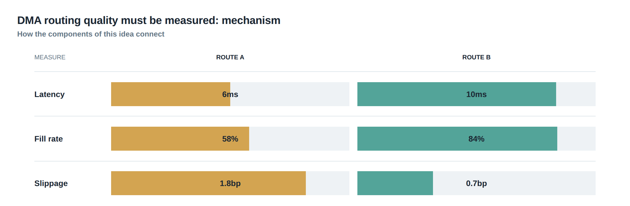
When an order is generated, the execution engine first consults a routing matrix that maps instrument identifiers to a ranked list of venues, each annotated with latency estimates, fee schedules, and historical queue‑performance metrics. The engine then selects the top‑ranked venue, opens a TCP/IP socket (or an SBE‑compatible UDP channel), and transmits the order packet. The venue’s matching engine immediately places the order in its price‑time priority queue, returning a sequence number that encodes the order’s position relative to existing resting orders.

Simultaneously, the desk’s market‑data feed updates the best‑bid/best‑ask (BBO) and depth‑of‑book (DoB) snapshot. If the incoming order sits behind a large volume of opposite‑side orders, the expected time to execution can exceed the algorithm’s target horizon. At this point the routing logic may decide to cancel and re‑route, but such a decision must be based on a quantitative assessment of queue value: the expected spread capture, the probability of adverse selection, and the option value of staying in line. The engine therefore recomputes an execution‑utility score in real time, balancing the cost of cancellation against the potential benefit of a fresher venue.

A worked example with real numbers

Consider a EUR/USD market‑making algorithm that decides to sell 1 million units at a decision price of 1.1050. The routing matrix lists Venue A (direct DMA, 30 µs round‑trip) and Venue B (indirect, 70 µs round‑trip) as candidates. Venue A’s order book shows 800 k at 1.1050 and a further 500 k at 1.1048. Venue B shows 300 k at 1.1050 and 900 k at 1.1049.

The engine selects Venue A because of the lower latency. The order arrives, is placed behind a 1.2 million‑unit queue at the 1.1050 price level, and receives an acknowledgement indicating a queue position of 2.2 seconds to full execution under current flow. After 0.8 seconds, the market moves 2 ticks lower, the BBO becomes 1.1048/1.1052, and the algorithm’s target horizon is 1.0 second. The execution‑utility model now estimates that remaining in the queue would cost an additional 4 bps of adverse‑selection risk, while cancelling and re‑routing to Venue B would add 70 µs of latency but provide access to 900 k at 1.1049, likely filling within 0.4 seconds.

The engine issues a cancellation at 0.8 seconds, records the cancellation outcome (partial fill of 200 k at 1.1050, 0.8 seconds elapsed), and re‑routes the remaining 800 k to Venue B. The new order arrives at 1.1050, takes the front of the queue, and is fully executed at 1.1049 within 0.35 seconds. The final fill price is therefore 1.1049, representing a 1 bp improvement over the hypothetical full‑fill price at Venue A (1.1050) and a 2 bp improvement over the decision price, after accounting for the 0.8 second partial execution cost.

This numeric illustration shows that the shortest network route can be inferior when it repeatedly joins a long queue, while a slightly slower path may deliver faster executable depth and a better overall execution quality.

Where it breaks in live markets

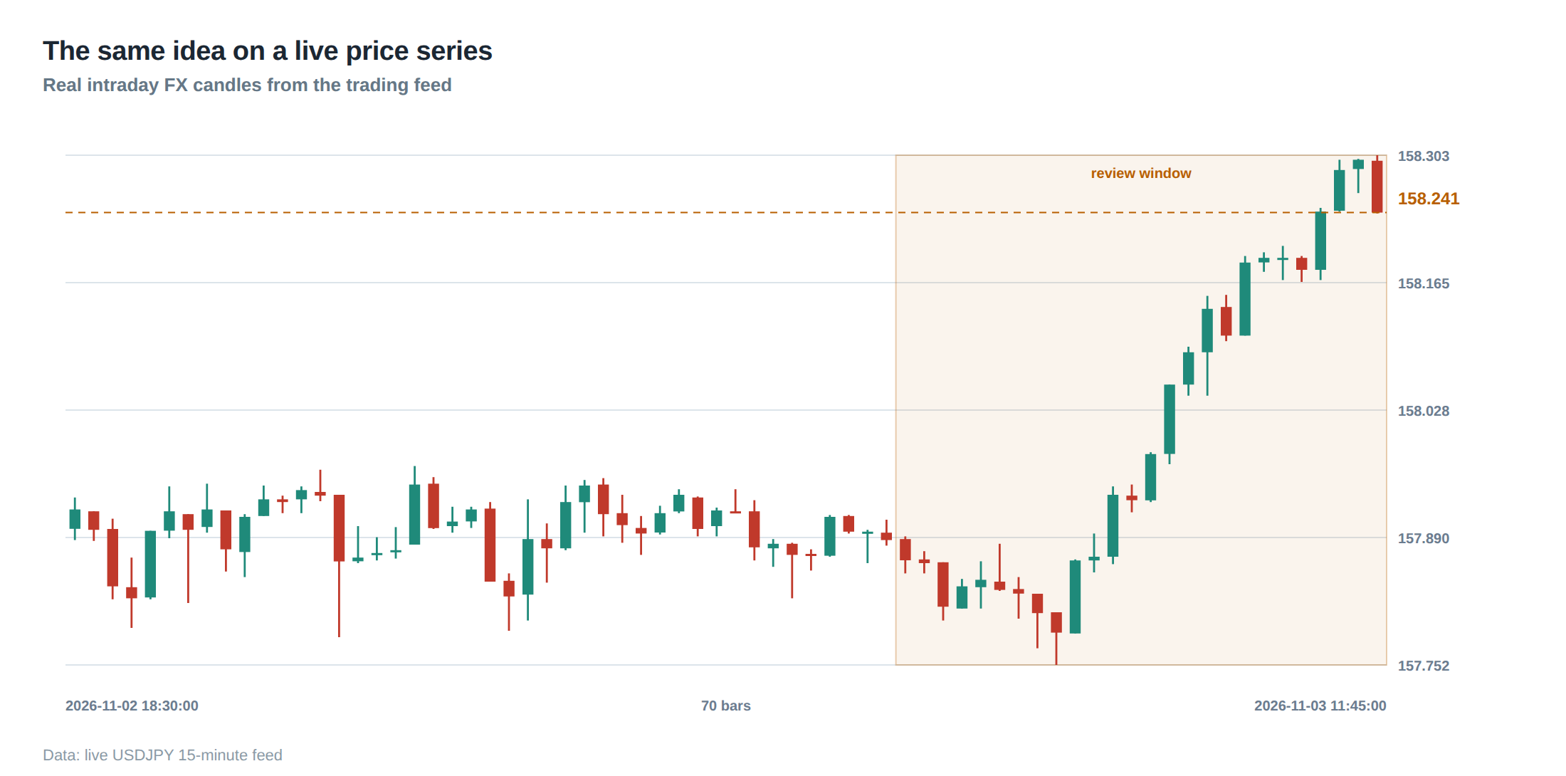
In live trading environments the assumptions that underpin static routing matrices decay rapidly. Venue‑level rule changes—such as the introduction of minimum order‑to‑display sizes, hidden order tiers, or dynamic fee structures—alter the effective depth that is visible to the algorithm. Moreover, sudden influxes of order flow from other participants can swell queues in milliseconds, turning a previously optimal venue into a bottleneck.

Latency spikes caused by network congestion or hardware contention further exacerbate the problem. A DMA line that normally delivers sub‑50 µs latency may experience micro‑bursts that push latency into the hundreds of microseconds, eroding the advantage over an indirect route that benefits from a more stable path. When these conditions coincide, the algorithm may continue to feed orders into a venue that appears optimal on paper but is, in reality, delivering worse price‑time outcomes.

The operating path, stage by stage

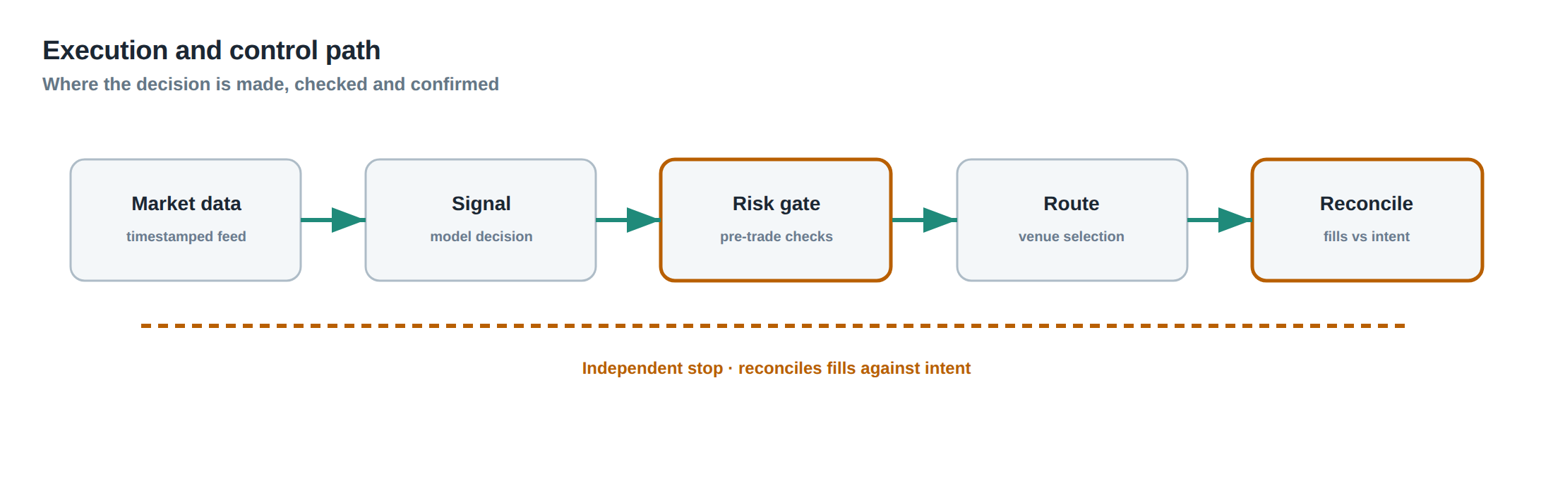
The execution pipeline can be divided into four logical stages. First, the decision layer evaluates market conditions and produces a trade intent, including the decision price and a target execution window. Second, the routing layer selects a venue based on the current routing matrix and transmits the order. Third, the venue response layer captures acknowledgements, queue positions, and any immediate market‑data changes that affect the order’s standing. Fourth, the evaluation layer continuously recomputes the execution‑utility score, deciding whether to let the order run to completion, to amend it, or to cancel and re‑route.

Each stage produces a timestamped log entry that, when chained together, yields a full audit trail from decision to final fill. The audit trail is essential for post‑trade analysis, allowing the desk to isolate the contribution of each component—network latency, venue queue dynamics, and routing logic—to the overall execution cost.

Controls that act before the damage

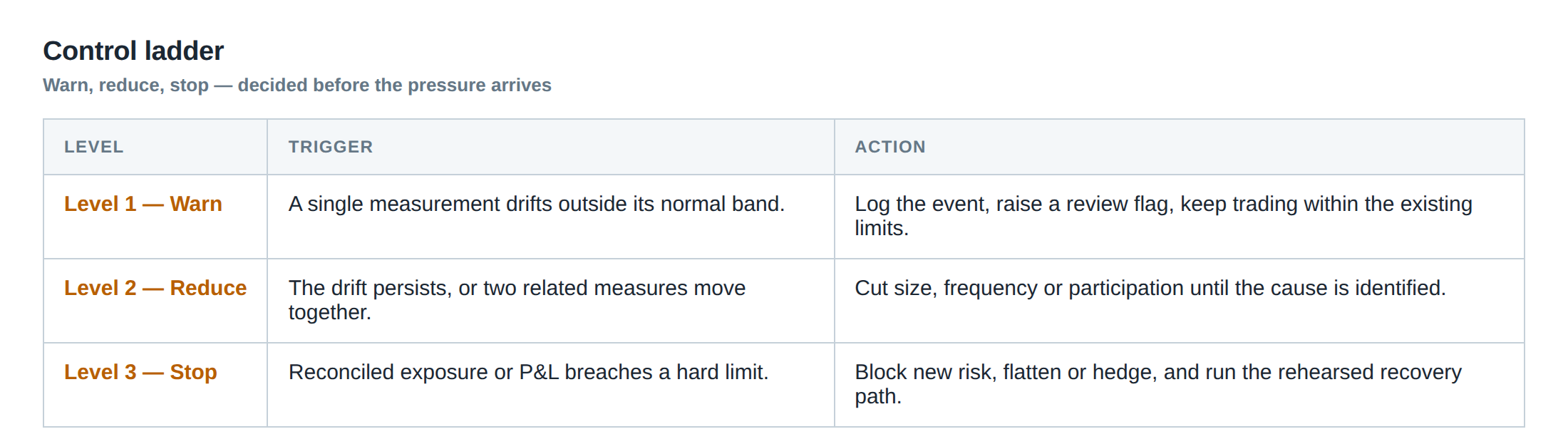
Preventative controls are built around early‑warning signals that flag deteriorating queue conditions. A “queue‑length threshold” monitors the depth at the intended price level and triggers a cancellation if the expected time‑to‑fill exceeds a configurable fraction of the target horizon. A “price‑movement guard” watches for BBO shifts that would render the original decision price sub‑optimal, prompting a re‑evaluation of the routing choice.

Another layer of protection is the “venue‑health monitor” that ingests latency statistics, packet loss rates, and venue‑specific status codes. When the monitor detects a sustained increase in round‑trip time beyond a pre‑set tolerance, it automatically demotes the affected venue in the routing matrix, forcing the engine to consider alternatives even if they are nominally slower. These controls act before a costly partial fill or a full‑fill at an adverse price can materialise.

How to measure whether it is working

Measurement must be anchored to the three‑point benchmark introduced earlier: decision price, arrival price, and final fill price. The primary metric is the “execution slippage” defined as the difference between arrival and decision prices, expressed in basis points. A secondary metric, “queue impact,” captures the spread captured or lost between arrival and final fill, adjusted for the proportion of the order that was filled at each price level.

Partial‑fill analysis adds granularity: for each slice of the order, record the time to completion and the price realised, then compute the average time‑to‑completion across all slices. Comparing this against the expected queue‑time model validates whether the routing logic is accurately forecasting queue dynamics. Finally, a “routing‑efficiency ratio” can be derived by dividing the realised execution slippage by the theoretical minimum slippage achievable on the same venue given the observed depth, providing a normalised view of routing performance.

The portfolio view

When the desk aggregates execution data across multiple instruments, patterns emerge that are invisible at the single‑order level. Certain venues may consistently under‑perform for high‑frequency, small‑lot trades but excel for larger, block‑size orders. Conversely, some DMA links may show sporadic latency spikes that only affect instruments with tight tick sizes.

By overlaying the execution‑utility scores with portfolio‑level risk metrics—such as realised P&L variance and turnover rate—the desk can adjust its routing matrix to align with strategic objectives, whether that be minimising transaction cost, reducing inventory risk, or preserving market‑making rebates. The key is to treat routing quality as a dynamic, portfolio‑wide optimisation problem rather than a static, per‑order decision.

In light of the evidence presented, how will you redesign your routing logic to account for queue dynamics and venue‑specific latency variations?

About the research behind this lesson

The seminar frames electronic markets as price-time-priority queues. It separates queue value into spread capture versus adverse-selection cost and the option value of retaining a place in line.

Applied to this lesson: An order lifetime therefore cannot be based on elapsed time alone: the system must reassess whether its queue position, expected spread and adverse-selection risk still justify keeping the order alive.

Two live systems, one desk

PULSE-X — power-packed HFT: high-frequency momentum on XAUUSD and EURUSD. System details · Live account

NIC-X — ultra-low drawdown: displaced-print arbitrage for large capital. System details · Live account

Start now: leave your email and request a free trial — we will send the pricing, the connection route and the trial terms. Pricing

Join the market discussion: Telegram @squawklive

Source: High-Frequency Trading and Modern Market Microstructure

Educational content only. Trading leveraged products involves risk.