October 7, 2026

What this problem really is

The term “drawdown” is often reduced to a single percentage printed on a performance screen, but that figure masks two distinct dimensions that matter to a prop‑trading desk. The first is the depth of the peak‑to‑trough loss, measured in absolute currency and as a proportion of capital. The second is the duration that capital remains below its previous high – the time‑under‑water. When a strategy suffers a 3 % loss over a single day, the impact on the balance sheet is very different from a 3 % loss that persists for three weeks while the market recovers.

At the strategy level the peak‑to‑trough metric tells the trader whether the model’s assumptions have been violated. At the portfolio level it tells the risk‑manager whether the overall capital buffer is being eroded faster than the firm can replenish it. A drawdown number that is not tied to any pre‑agreed response is therefore a passive observation rather than an active control. It can be ignored, or worse, it can be used as a trigger for an automatic increase in position size in the mistaken belief that “more capital will recover the loss faster”.

The core thesis is that a drawdown number becomes useful only when it is embedded in a hierarchy of actions – warning, de‑risking, and, if necessary, shutdown – and when the recovery process itself is governed by evidence rather than by a desire to chase losses. Only then does the metric serve as a lever for preserving optionality and protecting the firm’s capital base.

How the mechanism works, step by step

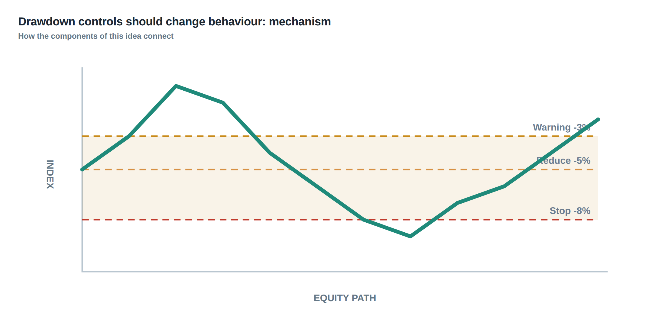
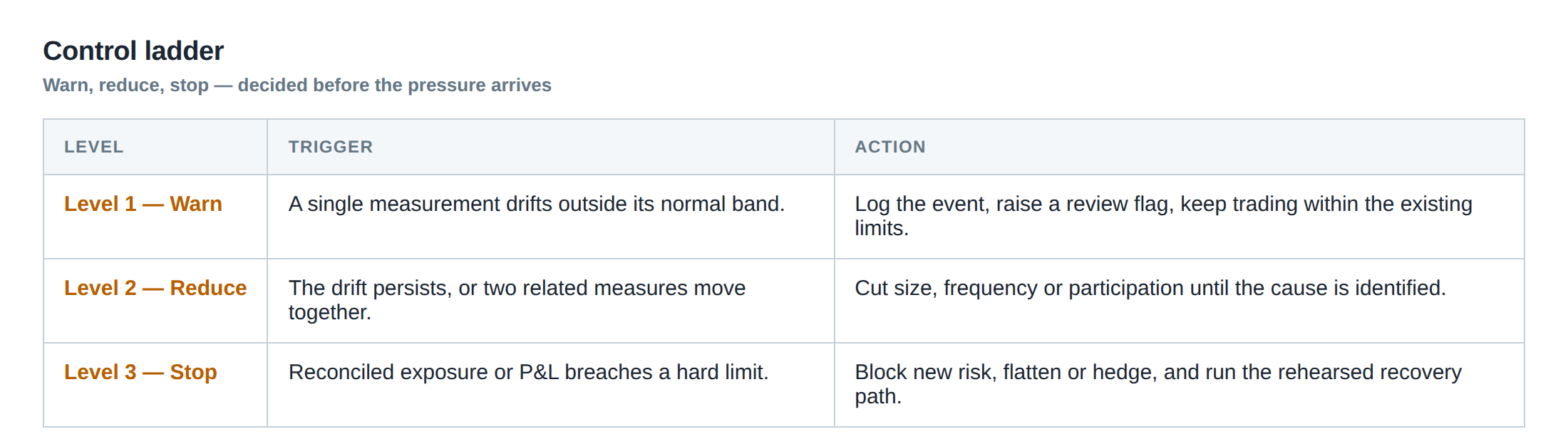
The first step is to define three quantitative thresholds that are applied consistently across all strategies. A warning threshold is set at a modest loss, for example 1 % of the strategy’s allocated capital, and it generates a real‑time alert to the trader and the risk‑desk. The second, a de‑risking threshold, is placed at a deeper loss – often 3–5 % – and it forces an immediate reduction in the risk budget, typically by cutting the maximum position size or the per‑trade volatility exposure in half. The third, a shutdown threshold, is a hard stop at a loss that would jeopardise the firm’s solvency, such as 10 % of the total portfolio, and it triggers a full suspension of the strategy until a post‑mortem is completed.

When a warning fires, the system records the event, timestamps the drawdown, and begins to monitor the subsequent behaviour of the strategy. If the loss continues to deepen, the de‑risking rule is executed automatically: the risk‑per‑trade parameter is scaled down, the order‑size multiplier is reduced, and any open positions are re‑evaluated against tighter stop‑losses. The shutdown rule is a final safeguard; it does not require a discretionary decision – the algorithmic gate simply rejects new orders once the loss exceeds the pre‑set limit.

Crucially, after a de‑risking event the trader must provide evidence that the underlying model has returned to statistical normality before the original risk budget is restored. Evidence can be a sequence of trades whose realised Sharpe ratio lies within one standard error of the model’s forecast, or a set of market‑microstructure metrics – latency distribution, fill‑rate stability, stale‑order frequency – that have returned to their baseline. Without such proof, the system keeps the reduced risk level, preserving optionality for when the market environment improves.

A worked example with real numbers

Consider a strategy that is allocated £10 million of capital and trades a medium‑frequency equity market‑making model. The original risk budget is 1 % of capital per trade, i.e. a maximum gross exposure of £100 000 per signal, with an expected daily volatility of 0.5 % and a target Sharpe of 2.0. The desk sets a warning threshold at a £200 000 (2 %) drawdown, a de‑risking threshold at £500 000 (5 %), and a shutdown threshold at £1 million (10 %).

During a volatile week the model suffers three consecutive losing trades of £80 000, £70 000 and £90 000 respectively. The cumulative loss reaches £240 000, crossing the warning line. An alert is raised, the risk‑monitor logs the event and the trader is asked to review order‑flow diagnostics. The loss continues, and after two more trades of £120 000 and £110 000 the total drawdown is £470 000, just shy of the de‑risking level. At this point the system automatically halves the per‑trade risk to 0.5 % of capital (£50 000) and tightens the stop‑loss from 2 % to 1 % of the position.

With the reduced exposure the next three trades produce modest gains of £30 000, £25 000 and £20 000, bringing the drawdown back to £395 000. The trader now submits a statistical report showing that the realised Sharpe over the last ten trades is 1.95, within the confidence interval of the model’s forecast. The risk‑desk, satisfied with the evidence, restores the original 1 % risk budget. The optionality preserved by the interim de‑risking step allowed the strategy to recover without breaching the shutdown limit.

Contrast this with an alternative response that some desks adopt: after the £470 000 loss the trader decides to double the position size to 2 % of capital in order to “make the money back faster”. The new per‑trade exposure becomes £200 000. The next two trades are again adverse, each losing £180 000, and the drawdown jumps to £830 000, now within the shutdown band. The system halts the strategy, but the capital loss is now irreversible; the original £10 million allocation has been reduced by more than 8 %, and the firm must re‑allocate resources from other desks to keep the strategy alive. The example demonstrates that a disciplined de‑risking rule protects optionality, whereas a reactive scaling‑up can turn a temporary model misspecification into a terminal event.

Where it breaks in live markets

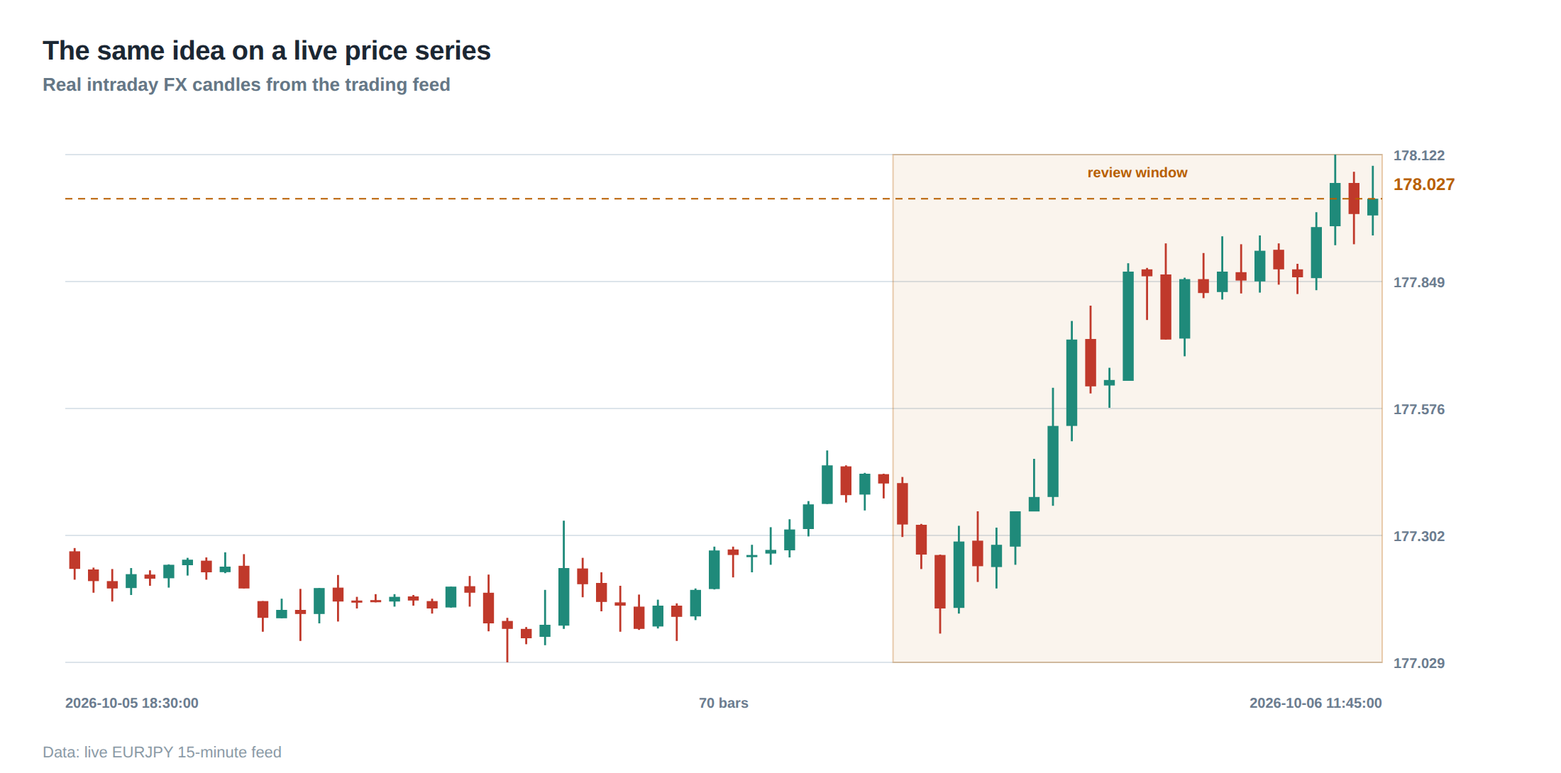
Even a perfectly calibrated set of thresholds can be bypassed when the market environment produces abnormal micro‑structure behaviour. Latency tails, for instance, are rarely captured by the average fill‑time statistic that most desks monitor. When a network outage adds a 200 ms tail to the latency distribution, orders that would normally be executed at the quoted price are now filled at a price that is, on average, three ticks worse. The resulting slippage pushes the realised loss distribution further into the tail, making drawdowns deeper and more frequent than the model predicts.

Stale‑order frequency is another hidden risk. A strategy that relies on a high‑frequency order‑book snapshot may continue to submit orders based on a price that has already moved. If the order‑cancellation engine lags, the market can move against the position before the order is withdrawn, creating a loss that is not reflected in the back‑tested return distribution. In such scenarios the warning threshold may be triggered by a single large loss that is actually a symptom of a routing failure, not a flaw in the predictive model.

Finally, automatic position scaling – the practice of increasing size after a loss to “recover faster” – defeats the very purpose of drawdown controls. The scaling rule is often coded as a simple function of cumulative loss, ignoring the fact that the loss may be due to a structural change in market dynamics. When the underlying statistical assumptions break, larger positions simply amplify the mis‑pricing and accelerate capital erosion. The drawdown metric, if not coupled with a requirement for evidence of model stability, becomes a trigger for self‑destructive behaviour.

The operating path, stage by stage

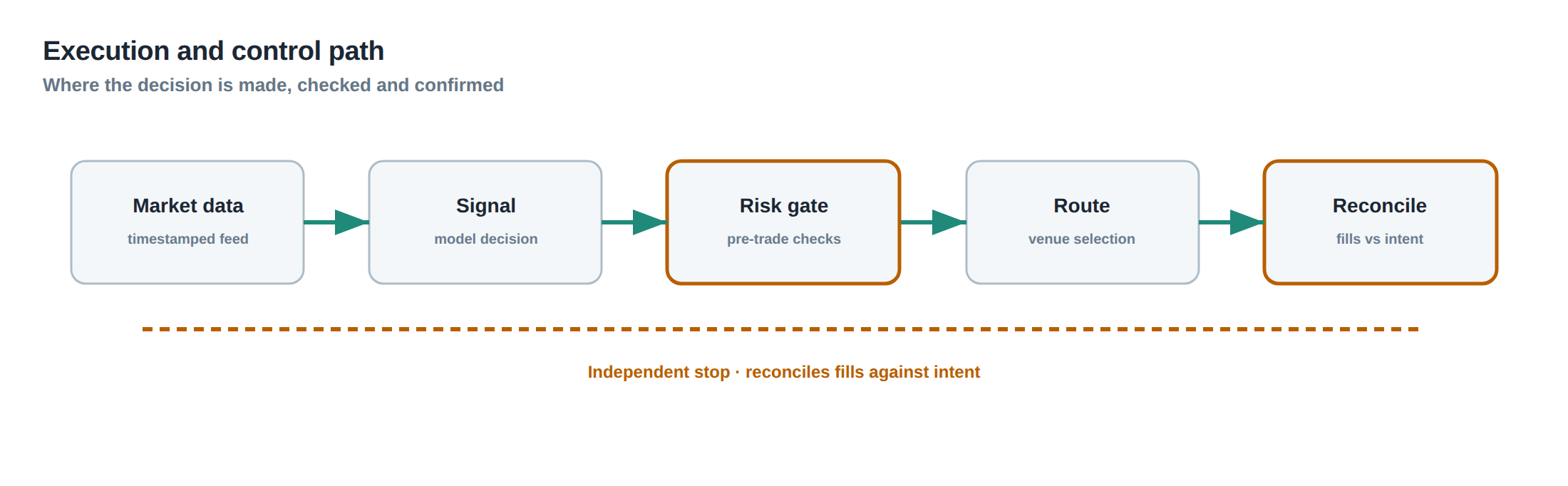
The control framework can be visualised as a sequential flow that starts with continuous monitoring and ends with post‑mortem analysis. First, a real‑time risk engine ingests trade‑level P&L, market‑data latency, and order‑execution quality, updating the peak‑to‑trough drawdown and the time‑under‑water for each strategy. Second, when the drawdown crosses the warning level, an alert is pushed to the trader’s dashboard and to the central risk‑monitoring screen; the alert includes the magnitude of the breach and the duration of the current underwater period.

Third, if the drawdown deepens to the de‑risking threshold, the engine automatically enforces a reduction in the risk‑budget parameters – the per‑trade volatility target, the maximum notional exposure, and the stop‑loss distance – without requiring manual confirmation. Fourth, the system logs the de‑risking event and opens a “recovery ticket” that the trader must close by providing statistical evidence of model health. Fifth, if the drawdown reaches the shutdown limit, the order‑gateway rejects any new orders from the strategy, and a suspension flag is raised on the portfolio‑allocation table. Sixth, after the suspension, a formal post‑mortem is conducted, the findings are recorded, and a decision is made whether to re‑activate the strategy with a fresh risk budget or to retire it permanently.

Each stage is designed to be auditable, with timestamps, parameter changes, and decision‑maker identifiers stored in an immutable log. The flow ensures that no human can bypass a de‑risking rule without leaving a trace, and that the recovery process is governed by data rather than by emotion.

Controls that act before the damage

Preventive controls sit upstream of the drawdown thresholds and aim to reduce the probability that a breach occurs in the first place. One such control is a dynamic position‑limit that scales with realised volatility: when the intraday realised volatility exceeds the model’s forecast by more than one standard deviation, the maximum notional size is automatically reduced by a preset factor. Another is a latency‑watchdog that monitors the 95th‑percentile round‑trip time; if the latency exceeds a pre‑defined ceiling, the strategy is paused until the network path is restored.

A ladder of pre‑trade checks also helps. The first rung verifies that the order price is within the current market spread; the second rung ensures that the order size does not breach the per‑trade risk budget; the third rung cross‑checks the aggregate exposure against the portfolio‑level capital utilisation limit. If any rung fails, the order is rejected before it reaches the market, eliminating the possibility of a sudden, large loss that could trigger a drawdown.

Risk‑budget allocation itself is a control. By assigning each strategy a fixed percentage of the total capital and by enforcing a hard cap on the sum of the individual risk budgets, the desk guarantees that a single strategy cannot consume a disproportionate share of the capital buffer. The ladder metaphor captures the idea that each control adds a layer of protection, and that the system only proceeds to the next layer when the previous one has been satisfied.

How to measure whether it is working

The effectiveness of the drawdown‑control framework is evaluated using a suite of quantitative diagnostics. The primary metric is the maximum drawdown (MDD) as a proportion of capital, measured both at the strategy and at the portfolio level. A secondary metric is the average time‑under‑water (ATUW), expressed in trading days, which captures how long capital remains below its previous high. A reduction in ATUW after the introduction of de‑risking rules indicates that the system is able to bring the capital back to peak more quickly.

Another useful indicator is the frequency of threshold breaches per annum. A high frequency of warning alerts but a low frequency of de‑risking or shutdown events suggests that the warning level is set too low, generating noise without adding protective value. Conversely, an absence of any breaches may indicate that the thresholds are set so conservatively that they never engage, potentially leaving optionality on the table.

Risk‑adjusted performance measures, such as the Calmar ratio (annual return divided by maximum drawdown) and the Sortino ratio (return divided by downside deviation), should be tracked before and after the implementation of the control framework. An improvement in these ratios, coupled with a stable or higher Sharpe ratio, demonstrates that the controls are not merely reducing risk at the cost of expected return, but are preserving the risk‑adjusted edge of the strategy.

Finally, post‑mortem analyses of any shutdown events provide qualitative evidence of the framework’s value. By documenting the root cause – for example, a latency spike or a model‑parameter drift – and the subsequent corrective actions, the desk builds a knowledge base that can be used to refine thresholds and preventive controls.

The portfolio view

At the portfolio level the drawdown control framework must reconcile the individual strategy limits with the overall capital‑budget policy. The aggregate peak‑to‑trough loss is not simply the sum of the individual drawdowns because correlations between strategies can either amplify or dampen the total loss. A portfolio‑wide stress test that applies simultaneous drawdowns to correlated strategies provides a realistic estimate of the worst‑case capital erosion.

Capital allocation is therefore performed on a risk‑budget basis: each strategy receives a risk‑budget that reflects its expected contribution to the portfolio’s overall volatility, its Sharpe ratio, and its drawdown profile. When a strategy breaches its de‑risking threshold, the freed risk budget can be re‑allocated to other strategies that are still within their warning band, preserving the portfolio’s ability to generate returns while protecting the capital base.

Time‑under‑water at the portfolio level is especially important for liquidity‑constrained desks. If the portfolio remains underwater for an extended period, the firm may be forced to liquidate positions at adverse prices to meet margin calls. Monitoring the portfolio ATUW alongside the individual strategy ATUWs enables the risk‑desk to intervene early, for example by re‑balancing the allocation or by temporarily tightening the risk budgets of all strategies.

In practice, the portfolio view is visualised on a dashboard that plots the cumulative equity curve, overlays the portfolio‑level warning, de‑risking, and shutdown thresholds, and displays the current risk‑budget utilisation as a percentage of the total capital. The dashboard also shows the contribution of each strategy to the current drawdown, allowing the desk to pinpoint which models are driving the loss and to apply targeted de‑risking actions.

The disciplined use of drawdown numbers, coupled with predefined actions and a controlled recovery process, transforms a passive risk statistic into an active lever for capital preservation. By measuring both depth and duration, enforcing a ladder of thresholds, preventing automatic scaling‑up, demanding statistical evidence before restoring full risk, and monitoring performance at the portfolio level, a prop‑trading desk can retain optionality while guarding against ruin.

Do you have a clear, documented process that ties every drawdown breach to a concrete, evidence‑based action plan?

About the research behind this lesson

Andrew Lo's lectures build risk analysis from return distributions and statistical measures, rather than treating one realised result as a complete description of risk.

Applied to this lesson: For a fast strategy, median latency or average fill quality is not enough. The review has to include tail delays, stale-order frequency and the loss distribution when cancellation or routing behaves abnormally.

Explore PULSE: System details

PULSE live account: Verify the live account on FX Blue

Live chat and updates: Telegram @xtrskhft

Source: Risk and Return

Educational content only. Trading leveraged products involves risk.