October 31, 2026

What this problem really is

A draw‑down is simply the distance between a portfolio’s highest equity point and the lowest point that follows before a new high is set. In practice the number is often quoted as a percentage – for example a 4 % peak‑to‑trough loss on a $20 m book – but the raw figure tells us nothing about the discipline that follows it. Without a pre‑agreed response, a draw‑down becomes a retrospective statistic rather than a forward‑looking control. The danger is that traders, eager to “make the money back”, will increase position size, tighten leverage or add new capital in the hope of a rapid rebound. Those actions are rarely justified by the underlying model and frequently turn a temporary under‑performance into a permanent capital loss.

The academic perspective that underpins modern risk management treats realised outcomes as samples from a distribution, not as the full description of risk. The emphasis is on the shape of the tail, on the probability of extreme moves, and on how those extremes interact with operational frictions such as latency spikes, stale‑order execution or abnormal routing. In a fast‑moving strategy, the median fill latency or average slippage is insufficient; the risk manager must also understand the frequency of outlier delays and the loss distribution when the execution chain behaves abnormally. The same philosophy should apply to draw‑down control – the policy must be built on statistical expectations, not on the hope that the next trade will simply reverse the loss.

When a desk treats draw‑down as a trigger for a set of actions – a warning, a de‑risking step, and, if necessary, a shutdown – the number ceases to be a passive metric and becomes an active lever. The lever can be calibrated to protect optionality, to keep the capital base intact, and to ensure that any recovery is driven by evidence that the model still works, rather than by desperation. The core thesis, therefore, is that a draw‑down figure is useful only when it is coupled to a predefined, enforceable process that governs both the reduction of risk and the conditions required before risk can be restored.

How the mechanism works, step by step

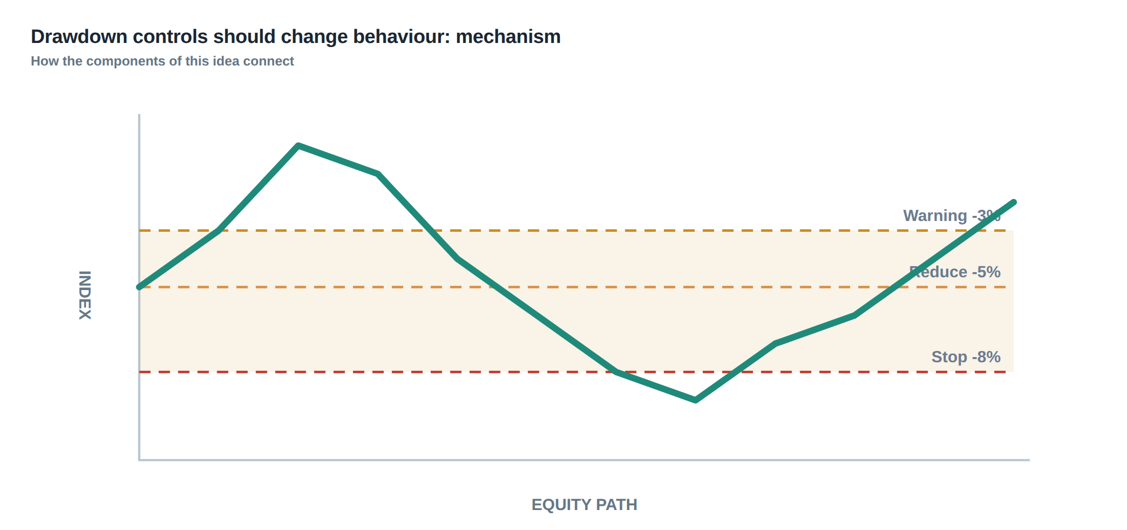
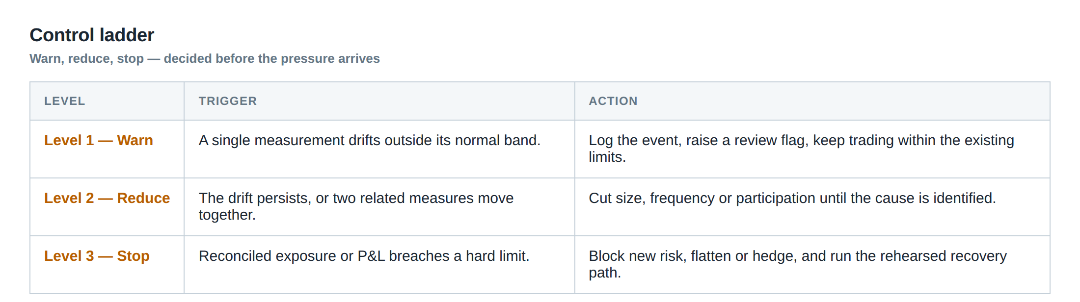
The first element of a robust draw‑down control is the definition of three thresholds: a warning level, a de‑risking level and a shutdown level. The warning level is typically set at a modest fraction of the total risk budget – for instance 1 % of capital – and serves as an early‑warning that the strategy is deviating from its expected return distribution. Once the equity curve falls below the de‑risking threshold, which might be 2 % or 3 % of capital, the system automatically scales the position‑size multiplier down by a pre‑specified factor, often 50 % of the original allocation. If the draw‑down deepens to the shutdown level, say 5 % of capital, the algorithm halts new order flow and flags the strategy for immediate review.

The scaling action is not a discretionary decision taken by a trader in the heat of the moment. It is encoded in the order‑routing logic so that, as soon as the equity curve breaches the de‑risking line, the risk‑per‑trade parameter is recomputed and all subsequent orders are sent with the reduced size. This prevents the common behavioural bias of “doubling down” to recover losses. The system also records the time spent underwater – the duration between the high and the next new high – because a shallow but prolonged draw‑down can be more damaging to capital than a deep, brief dip.

Restoring full risk after a shutdown is a separate, evidence‑based process. The desk must first verify that the statistical properties of the strategy – mean return, volatility, tail risk – remain within the confidence intervals established during back‑testing and live‑paper. Only after a series of qualifying trades, with realised performance consistent with the model, does the risk‑per‑trade parameter revert to its original level. This staged restoration guards against premature re‑exposure that could amplify a model breakdown into a catastrophic loss.

A worked example with real numbers

Consider a proprietary fund that allocates $10 million to a high‑frequency statistical arbitrage strategy. The baseline risk budget is 1 % of capital per day, which translates to a maximum daily exposure of $100 000. The strategy’s historical daily return distribution has a mean of 0.12 % and a standard deviation of 0.8 %, with a 99 % VaR of –2.1 %. The desk sets a warning threshold at a 1 % draw‑down ($100 000), a de‑risking threshold at 2 % ($200 000) and a shutdown threshold at 5 % ($500 000).

On day 12 the equity curve falls to $9.85 million, a 1.5 % draw‑down. The warning line is breached, but the de‑risking line is not yet reached, so the system logs the event and continues trading at the full $100 k daily exposure. Two days later the draw‑down deepens to $9.70 million – a 3 % loss – crossing the de‑risking threshold. The automated controller instantly halves the daily risk budget to $50 k. Over the next five days the strategy generates modest positive returns, lifting equity to $9.78 million, still below the original high. Because the draw‑down remains under the shutdown level, trading continues at the reduced size.

Suppose instead that after the 3 % dip the trader, convinced that the market will revert, decides to double the position size to $200 k in an attempt to accelerate recovery. The next three days see a series of adverse fills and a latency spike that pushes the realised loss to an additional $300 k, pushing the total draw‑down to 6 % and triggering the shutdown condition. The strategy is halted, and the capital base is now $9.4 million. The subsequent review discovers that the model’s assumptions about mean reversion have broken down under the heightened market volatility, a fact that would have been evident had the original de‑risking rule been respected. The premature scaling not only failed to recover the loss but also exposed the fund to a ruin scenario that the original risk‑budget design was meant to avoid.

This example illustrates two key points. First, a modest reduction in exposure after a predefined draw‑down preserves optionality – the fund retains capital to exploit future favourable moves without over‑committing. Second, an aggressive size increase can transform a temporary model miss‑specification into a permanent capital erosion, confirming the thesis that draw‑down numbers are only useful when they are tied to enforceable actions.

Where it breaks in live markets

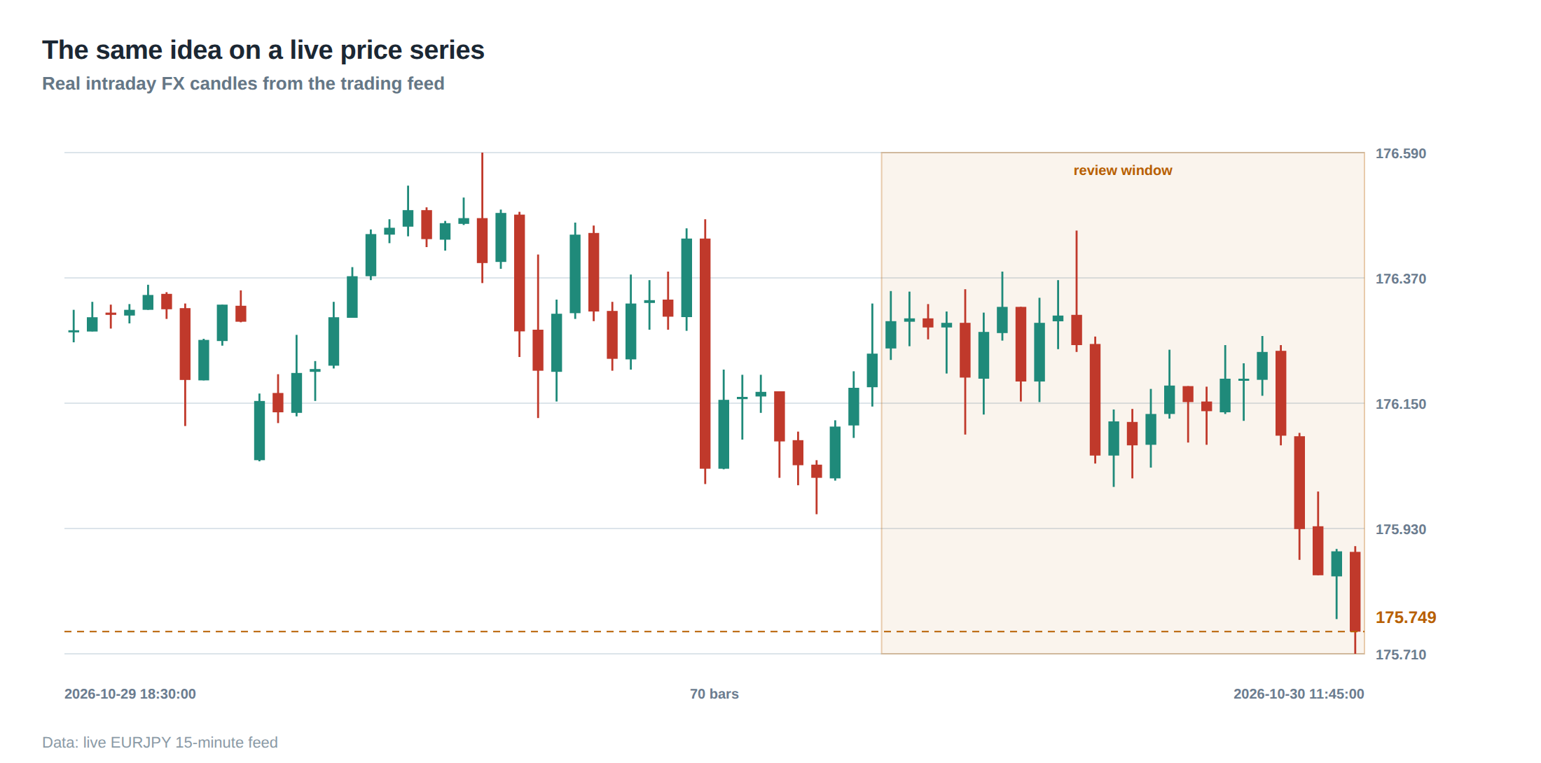
Even a perfectly specified draw‑down ladder can be undermined by operational realities. In live trading, latency is not a static figure; network congestion, exchange outages and routing anomalies create occasional spikes that push execution times into the tail of the distribution. When a latency event coincides with a market move, the realised loss can be far larger than the statistical VaR predicts, causing the equity curve to breach the shutdown threshold before the monitoring system can react.

Stale orders present another failure mode. If the order‑book reference becomes outdated – for example because the market microstructure has shifted faster than the order‑generation engine can adapt – the strategy may submit prices that are no longer executable. The resulting cancellations and re‑submissions generate additional transaction costs and can leave the position partially filled, exposing the desk to asymmetric risk. In such scenarios the draw‑down control may be triggered by the loss of the intended hedge rather than by market movement per se, and the subsequent de‑risking may not be sufficient if the underlying exposure remains hidden in the order book.

A third source of breakdown is the human tendency to override automated limits. If a senior trader believes that a particular market regime favours a larger position, they may manually lift the de‑risking multiplier, effectively bypassing the control. Unless the system logs and audits every such override, the desk loses the ability to attribute subsequent performance to the original risk framework, and the protective intent of the draw‑down ladder is eroded.

Finally, the interaction between multiple strategies can generate correlated draw‑downs that exceed the sum of their individual thresholds. If two statistically independent strategies happen to be exposed to the same liquidity shock, their simultaneous losses can push the aggregate portfolio past the shutdown level even though each strategy individually remains within its own limits. Without a portfolio‑wide monitoring layer, the desk may be blindsided by a systemic event that the per‑strategy draw‑down controls alone cannot contain.

The operating path, stage by stage

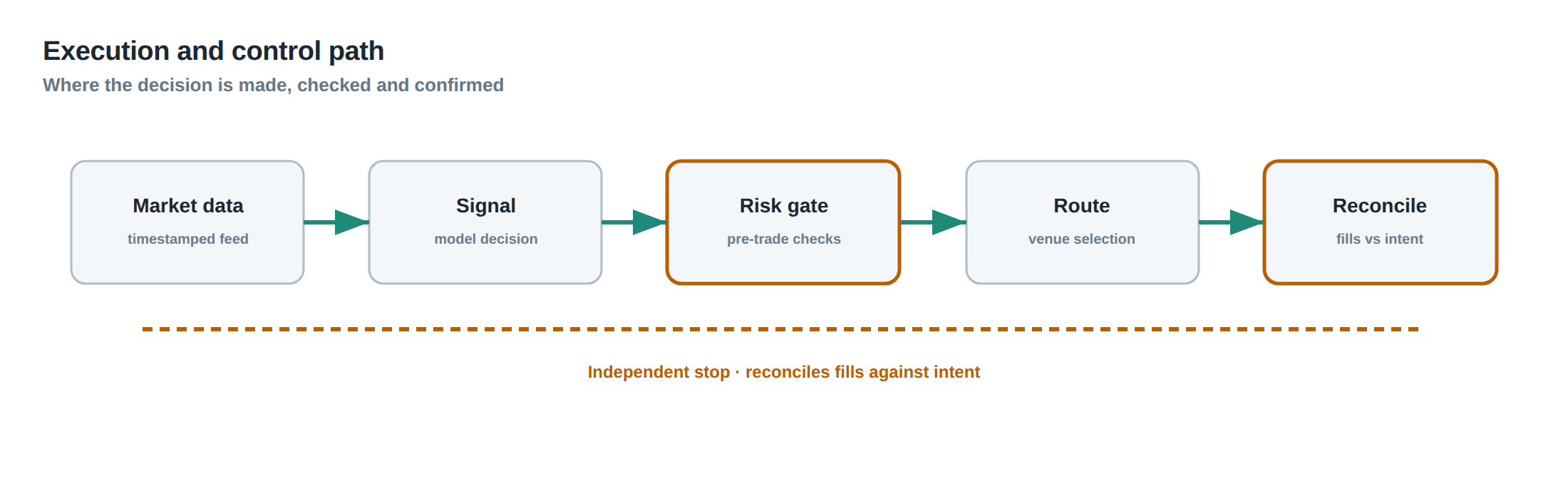
The first stage of the operating path is continuous equity‑curve monitoring. A high‑frequency data feed records the cumulative profit and loss at sub‑second granularity, feeding a rolling maximum tracker that identifies the current peak. The second stage is threshold evaluation. As soon as the difference between the peak and the current equity exceeds the warning level, an alert is generated and logged; the trader desk receives a visual cue but trading proceeds unchanged.

The third stage is the de‑risking trigger. When the draw‑down passes the de‑risking line, a risk‑engine routine recalculates the per‑trade exposure limit, applying the pre‑defined reduction factor. All order‑generation modules query this limit before transmitting a new order, ensuring that the reduced size is enforced in real time. The fourth stage is the shutdown protocol. If the equity curve falls to the shutdown threshold, the order gateway is instructed to reject any new orders, and the existing positions are either flat‑lined or hedged according to a pre‑approved unwind schedule.

Stage five involves a post‑mortem review. A risk analyst extracts the trade log, execution timestamps, and market microstructure data for the period of the draw‑down. The analyst tests whether the loss distribution during the event aligns with the model’s tail expectations, and whether any operational anomalies – latency spikes, stale orders, routing failures – contributed materially. The sixth stage is the evidence‑based restoration. Only after the analyst signs off on a set of qualifying trades that demonstrate the model’s statistical properties are the original risk limits reinstated, and the system returns to the monitoring state.

Each of these stages is designed to be deterministic and auditable, removing discretionary judgement from the moment a draw‑down is observed. The flow from detection to action, and back to normal operation, forms a closed loop that safeguards capital while still allowing the strategy to resume once confidence is restored.

Controls that act before the damage

Preventive controls sit upstream of the draw‑down ladder and aim to reduce the probability that the equity curve ever reaches a critical level. The first line of defence is a pre‑trade risk filter that checks the projected exposure against a daily risk budget, a maximum position‑size cap, and a concentration limit across correlated instruments. If any of these checks fail, the order is rejected before it reaches the market.

A second preventive measure is dynamic position sizing based on real‑time volatility estimates. By scaling exposure inversely with realised volatility, the system automatically reduces risk during turbulent periods, thereby lowering the likelihood of a rapid equity decline. This volatility‑adjusted sizing is recomputed for each new market snapshot, ensuring that the risk budget adapts to the current market regime rather than remaining static.

The third control is a latency‑budget guard. The execution engine monitors the round‑trip time of each order; if the latency exceeds a pre‑set percentile of the historical distribution – for example the 95 th percentile – the engine temporarily suspends order submission for that instrument. This prevents the strategy from entering a market when execution quality is degraded, a situation that historically correlates with larger than expected losses.

Finally, a capital‑allocation ladder is maintained at the portfolio level. Each strategy is assigned a maximum draw‑down budget that, when summed across the portfolio, does not exceed a predefined fraction of total capital. This ensures that a single strategy’s loss cannot consume the entire risk budget, preserving optionality for the remaining strategies. Together, these upstream controls create a buffer that reduces the frequency and severity of draw‑downs, making the downstream ladder a safety net rather than a primary defence.

How to measure whether it is working

Effectiveness is assessed by two complementary metrics: the frequency of threshold breaches and the recovery profile after each breach. A well‑tuned system should exhibit a low incidence of shutdown events – ideally less than one per quarter for a mature strategy – while maintaining a reasonable number of warning alerts that serve as early‑stage diagnostic signals. The average time spent underwater after a de‑risking event should be measured in days rather than hours, indicating that the reduced exposure is allowing the equity curve to stabilise before attempting a recovery.

Another key indicator is the optionality preserved. By comparing the realised capital at the end of a draw‑down episode with the hypothetical capital trajectory that would have resulted from an aggressive size increase, the desk can quantify the cost of restraint versus the cost of ruin. In the worked example, halving exposure after a 3 % draw‑down preserved $200 k of capital that would have been lost had the position been doubled, a tangible demonstration of the control’s value.

A third measurement is the alignment of realised loss distribution with the model’s tail expectations during draw‑down periods. Statistical tests such as the Kolmogorov–Smirnov distance between the empirical loss distribution and the calibrated model distribution provide an objective gauge of whether the strategy’s behaviour remains consistent with its risk assumptions. If the distance widens significantly during a draw‑down, the evidence‑based restoration process should be delayed.

Finally, audit logs of every automatic risk‑limit change, together with timestamps of alerts, provide a traceable record that can be reviewed by senior risk officers. The completeness and timeliness of these logs are themselves a performance metric; any lag between a threshold breach and the corresponding risk adjustment indicates a weakness in the operating path that must be remedied.

The portfolio view

At the portfolio level, draw‑down controls must be coordinated across all active strategies to avoid unintended concentration of risk. The aggregate equity curve is monitored for a portfolio‑wide peak‑to‑trough loss, and a separate set of thresholds – often tighter than the per‑strategy limits – is applied to the total capital. When the portfolio draw‑down reaches its de‑risking level, the system may proportionally scale down exposure across all strategies, preserving the relative risk allocation while protecting the overall capital base.

Correlation analysis plays a crucial role. By continuously estimating the covariance matrix of strategy returns, the desk can identify periods when normally uncorrelated strategies become positively linked, for example during market stress. In such periods the portfolio draw‑down ladder can be tightened, lowering the de‑risking and shutdown thresholds to reflect the heightened systemic risk.

Capital budgeting also benefits from the time‑under‑water metric. Strategies that spend a long time underwater consume capital that could otherwise be deployed to higher‑conviction ideas. By assigning a cost to each day spent below the peak, the portfolio manager can prioritise the reallocation of capital away from under‑performing strategies once they have demonstrated a statistically significant recovery.

Ultimately, the portfolio view treats draw‑down control not as a series of isolated safety valves but as an integrated component of capital allocation, risk budgeting, and performance attribution. When each strategy’s draw‑down ladder is aligned with the portfolio‑wide safeguards, the desk can sustain a higher level of aggregate risk without jeopardising the firm’s solvency, and can do so with a clear, evidence‑based process that links every loss figure to a concrete, pre‑agreed action.

How will you embed draw‑down‑triggered actions into your own risk framework?

About the research behind this lesson

Andrew Lo's lectures build risk analysis from return distributions and statistical measures, rather than treating one realised result as a complete description of risk.

Applied to this lesson: For a fast strategy, median latency or average fill quality is not enough. The review has to include tail delays, stale-order frequency and the loss distribution when cancellation or routing behaves abnormally.

Two live systems, one desk

PULSE-X — power-packed HFT: high-frequency momentum on XAUUSD and EURUSD. System details · Live account

NIC-X — ultra-low drawdown: displaced-print arbitrage for large capital. System details · Live account

Start now: leave your email and request a free trial — we will send the pricing, the connection route and the trial terms. Pricing

Join the market discussion: Telegram @squawklive

Source: Risk and Return

Educational content only. Trading leveraged products involves risk.