October 17, 2026

What this problem really is

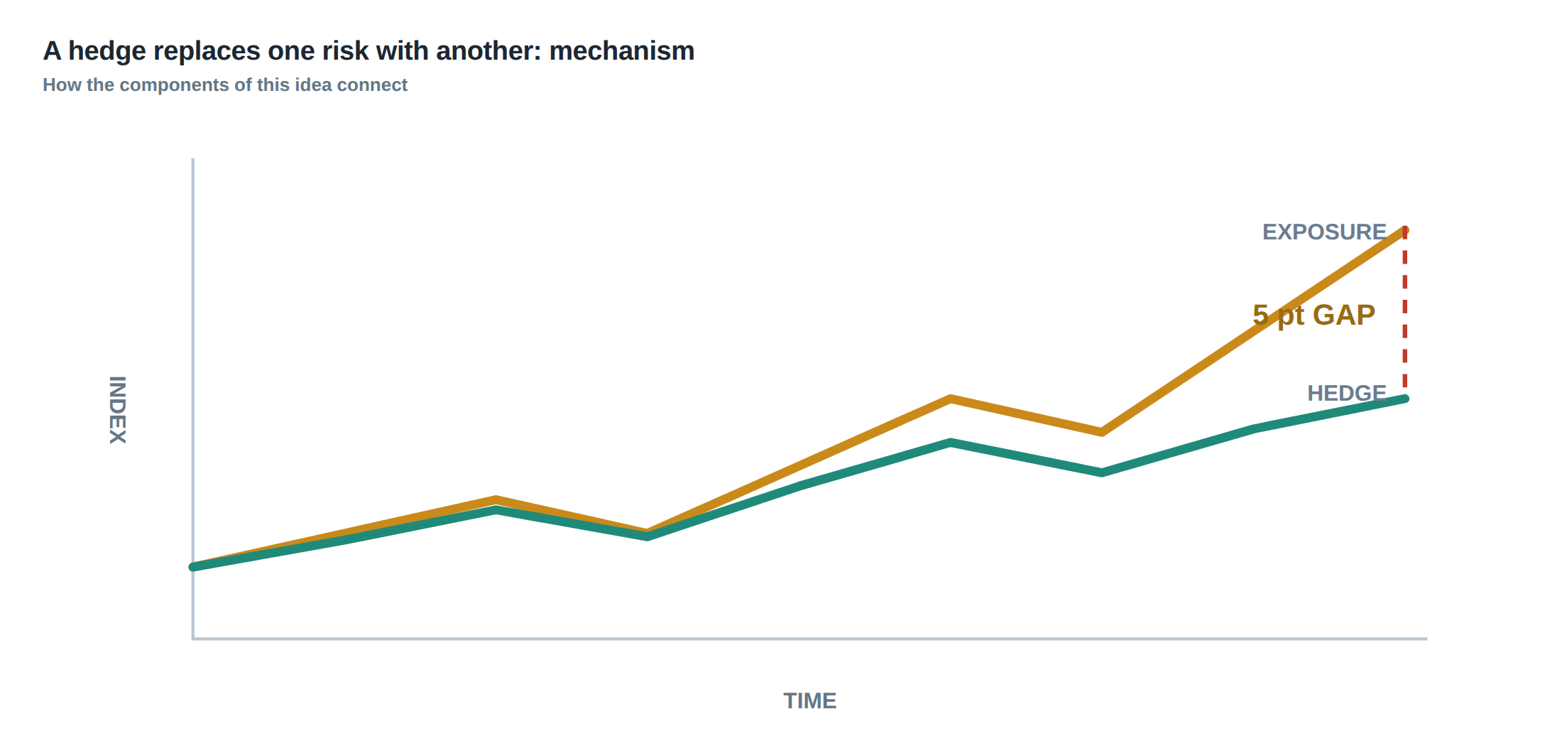
The instinctive view of a hedge is that it simply “takes away” a risk that the trader does not wish to own. In practice the operation replaces the original exposure with a new set of contingencies that are often less visible. The primary exposure – for example the equity‑index beta of a long‑only book – is swapped for the basis risk between the underlying and the proxy, the execution risk of placing the hedge order, the liquidity risk of maintaining the position over time, and the model risk inherent in the statistical relationship that underpins the hedge ratio. When the proxy diverges, the hedge can become a source of loss rather than protection. The net effect is a transformation of risk, not its elimination.

A useful way to think about the transformation is to view the hedge as a contract that obliges the desk to deliver or receive cash flows that are a linear combination of market variables. Those cash flows are priced, funded and rolled, and each of those steps introduces its own stochastic component. The resulting distribution of portfolio returns therefore contains the original market risk, the hedge‑specific risk, and the interaction between them. Ignoring any of those components creates a blind spot that can be exposed in periods of stress, when correlations break, spreads widen, or funding dries up.

How the mechanism works, step by step

The first step is to define the factor that the desk wishes to neutralise. In a typical equity‑index long book the factor is the systematic beta to the broad market, measured as the regression coefficient of the portfolio’s excess returns on the index’s excess returns over a look‑back window. Once the factor is identified, the hedge ratio is estimated – usually as the product of the target beta and the inverse of the estimated beta of the proxy instrument. The estimation itself carries sampling error; standard errors can be derived from the regression t‑statistics and from the variance of the residuals.

Having obtained a point estimate, the desk must decide how much of that estimate to trust. A common practice is to shrink the ratio toward zero by a factor proportional to its standard error, thereby limiting the size of the hedge when the statistical confidence is low. The next step is execution: the hedge order is sent to the market, often split across venues to minimise impact. After the trade clears, the desk records the realised hedge ratio, the execution price, and any slippage. From that moment onward the hedge is monitored for basis drift – the difference between the realised exposure of the proxy and the intended exposure – and for financing costs associated with the futures or swaps used to implement the hedge.

A worked example with real numbers

Consider a prop desk that manages a €100 million long exposure to the Euro Stoxx 50 index. The desk wishes to reduce its systematic beta from 1.00 to 0.30. A natural proxy is the E‑mini S&P 500 futures contract, which trades in US dollars and is highly liquid. Over the previous 250 trading days the regression of the Euro Stoxx 50 excess returns on the S&P 500 excess returns yields a beta of 0.85 with a standard error of 0.07 and a correlation of 0.92. The target hedge ratio is therefore

\[ \text{Hedge Ratio}=0.30 / 0.85 \approx 0.353 . \]

To account for estimation error the desk applies a 20 % shrinkage, arriving at a practical ratio of 0.28 futures contracts per €1 million of exposure, i.e. 28 contracts in total. The market price of the S&P 500 futures at the time of execution is 4 500 points, each point representing $50, so the notional of one contract is $225 000. Converting the €100 million exposure at an EUR/USD rate of 1.10 gives a USD equivalent of $110 million, requiring a notional of $30.8 million in futures, or 137 contracts. The desk therefore executes 28 % of that, i.e. 38 contracts, to achieve the shrunk hedge.

Execution incurs a slippage of 3 bps, costing €30 000, and the order is partially rejected on two venues, leaving a shortfall of 4 contracts (≈ 1 % of the intended hedge). The financing cost of holding the futures is the implied repo rate of 0.5 % per annum, while the desk must roll the contract each quarter at an estimated cost of 0.2 % of notional. Over a six‑month horizon the total hedge cost is therefore roughly €150 000. In calm market conditions the hedge reduces the portfolio’s one‑day VaR from €1.2 million to €0.4 million, a 66 % reduction in directional risk.

During a market shock – for example a sudden Euro‑dollar devaluation combined with a US equity sell‑off – the correlation between the two indices drops to 0.60 and the spread between the Euro Stoxx 50 futures and the spot widens by 150 bps. The hedge’s effective beta falls to 0.12, and the residual exposure to the original index rises to 0.18. The realised loss on the hedge, after accounting for the widened spread and the missed contracts, is €800 000, erasing most of the VaR benefit and leaving the desk with a net loss larger than the un‑hedged position would have suffered.

Where it breaks in live markets

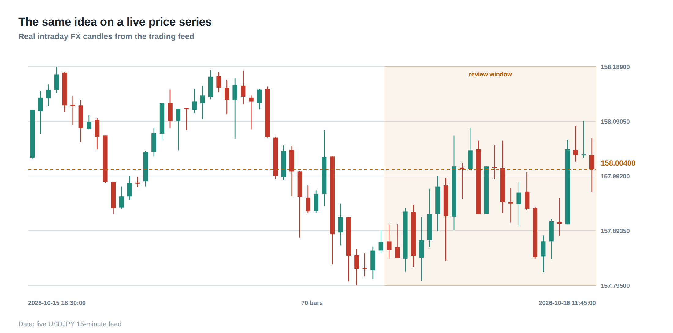
The theoretical construction assumes that the statistical relationship between the underlying and the proxy is stable, that execution is frictionless, and that financing conditions remain unchanged. In practice each of those assumptions is fragile. The research underpinning modern risk analysis demonstrates that a single realised outcome cannot capture the full distribution of possible losses; instead one must examine the entire return distribution, including its tails, to understand exposure. For a fast‑moving strategy, median latency or average fill quality is insufficient – the tail of the latency distribution, the frequency of stale orders, and the loss distribution when routing fails must be quantified.

When market stress hits, the beta estimate can shift dramatically, as observed when the Euro Stoxx 50 and the S&P 500 decouple during sovereign debt crises. Basis risk can explode because futures on the proxy may become illiquid, widening spreads and increasing the cost of rolling. Funding pressures can raise the implied repo rate, turning a cheap hedge into a costly liability. Execution risk also intensifies: order rejections rise, market depth evaporates, and slippage can climb from a few basis points to several hundred. These dynamics turn the hedge from a risk‑mitigating device into a source of model, liquidity, and execution risk that can dominate the portfolio’s loss profile.

The operating path, stage by stage

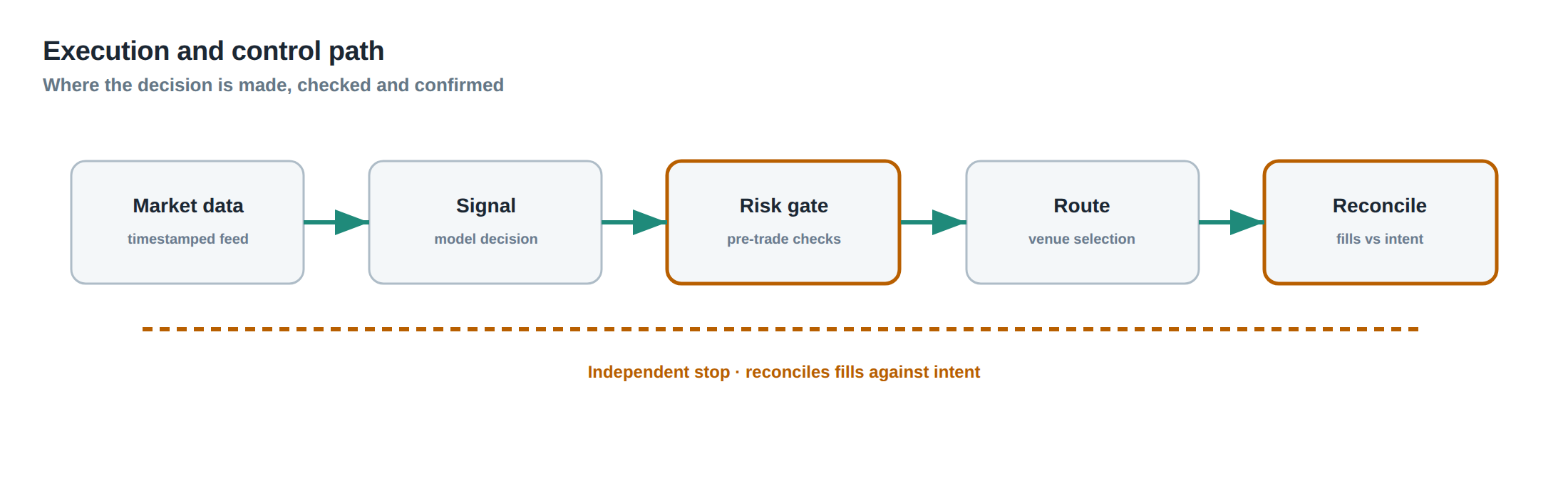
The first stage is identification – the desk selects the factor to hedge and chooses a proxy instrument that is liquid, tradable, and has a statistically significant relationship. The second stage is calibration – the hedge ratio is estimated, its confidence interval is computed, and any shrinkage or risk‑budget adjustments are applied. The third stage is execution – the order is sliced, routed, and monitored for fill quality, with any partial fills or rejections recorded for later reconciliation. The fourth stage is maintenance – the hedge is rolled, financing costs are accrued, and the realised hedge ratio is compared against the target on a daily basis. The final stage is unwind – when the exposure is closed or the hedge is no longer needed, the position is offset, and the net P&L of the hedge is realised.

Each stage has decision points that can be automated or overseen manually. For example, the calibration stage may trigger a review if the standard error of the beta exceeds a pre‑set threshold, prompting the desk to either increase shrinkage or seek an alternative proxy. The execution stage may invoke a fallback venue if the primary exchange rejects more than a defined proportion of the order. The maintenance stage may require a re‑estimation of the hedge ratio if the basis exceeds a tolerance band for three consecutive days. By structuring the process into discrete, observable steps, the desk can embed controls that detect deviations before they propagate into material loss.

Controls that act before the damage

Before the hedge is placed, the desk runs a pre‑trade risk check that validates the statistical significance of the proxy relationship, enforces a maximum allowable hedge size relative to the portfolio’s total capital, and confirms that funding for the futures is available at the expected repo rate. During the trade, a real‑time monitor tracks order acknowledgement latency, fills per venue, and the evolving slippage; any breach of the latency threshold raises an alarm that can pause further order flow. After execution, a reconciliation engine compares the intended hedge ratio with the realised one, flagging any shortfall beyond a pre‑defined basis tolerance.

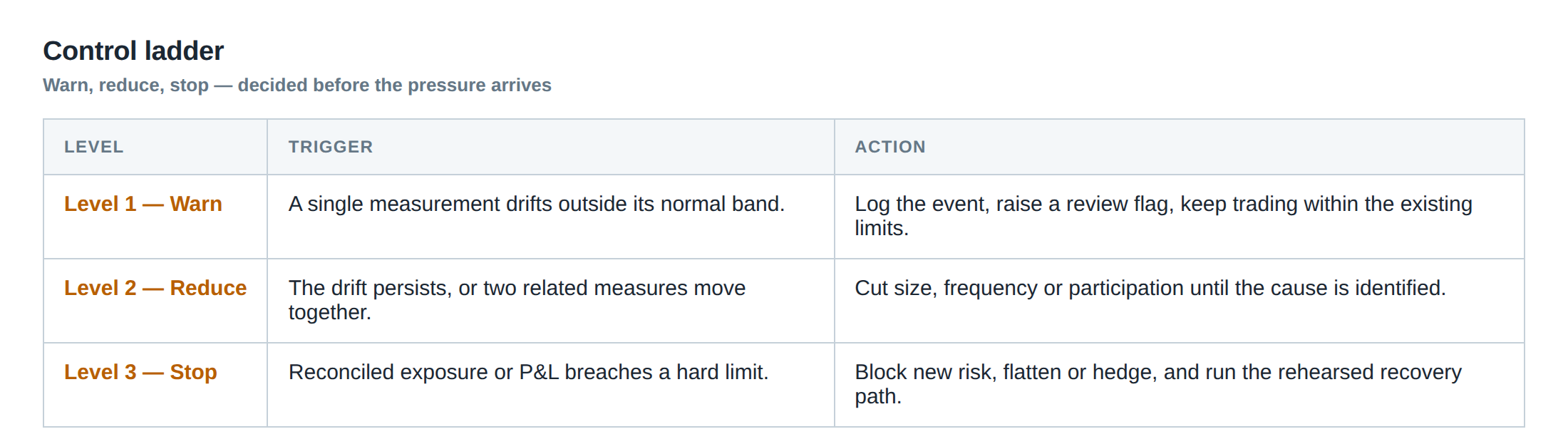
In the maintenance window, the desk runs a basis‑drift model that projects the expected spread between the proxy and the underlying under current market conditions. If the observed spread deviates from the model by more than two standard deviations, the system automatically initiates a hedge‑adjustment workflow, which may involve reducing the hedge size, switching to a different proxy, or adding a secondary hedge to cover the residual exposure. The ladder of controls – from statistical validation, through execution surveillance, to post‑trade reconciliation and ongoing drift detection – creates a layered defence that aims to catch the risk transformation early, before it materialises as a loss.

How to measure whether it is working

Effectiveness is measured by tracking the hedge’s reduction in portfolio variance and its contribution to tail risk. The primary metric is the hedge‑effectiveness ratio, computed as the proportion of variance in the portfolio’s returns that is explained by the proxy’s returns, typically derived from the R² of the regression. A secondary metric is the tracking error, the standard deviation of the difference between the portfolio’s realised exposure and the intended exposure after the hedge.

In addition, the desk monitors the realised cost of the hedge – financing, roll, and execution – against the expected cost budget. The distribution of daily P&L from the hedge is examined for skewness and kurtosis; an increase in negative skew or excess kurtosis signals that the hedge is contributing to tail risk rather than mitigating it. Finally, stress‑testing is performed by shocking the correlation and spread parameters to historic crisis levels and observing the resulting VaR and expected shortfall. If the hedge fails to contain losses under those scenarios, the hedge design is deemed insufficient.

The portfolio view

When the hedge is in place, the portfolio’s net exposure is the sum of the original systematic beta and the residual beta left after hedge implementation. In the worked example the original €100 million exposure with a beta of 1.00 is reduced to an effective beta of roughly 0.30 in normal markets, but during stress the residual beta may rise to 0.18 as the proxy relationship deteriorates. The portfolio’s risk budget must therefore allocate capital not only to the residual systematic exposure but also to the basis and execution risks introduced by the hedge.

Liquidity risk is reflected in the amount of capital reserved for potential roll‑over losses and for the possibility of having to unwind the hedge in an illiquid market. Model risk is captured by the confidence interval of the hedge ratio and the frequency of re‑estimation. By aggregating these components, the desk obtains a holistic view of the portfolio’s risk profile that recognises the hedge as a transformation of risk rather than its removal.

In practice, the desk reports a consolidated risk‑adjusted return that incorporates the hedge’s cost, its effectiveness, and the residual tail risk. The goal is to achieve a higher Sharpe ratio than the un‑hedged portfolio while maintaining a controlled level of extreme loss probability.

Do you have a systematic process for detecting when a hedge’s statistical relationship begins to break down, and how quickly can you act before the basis widens into a material loss?

About the research behind this lesson

Andrew Lo's lectures build risk analysis from return distributions and statistical measures, rather than treating one realised result as a complete description of risk.

Applied to this lesson: For a fast strategy, median latency or average fill quality is not enough. The review has to include tail delays, stale-order frequency and the loss distribution when cancellation or routing behaves abnormally.

Explore PULSE: System details

PULSE live account: Verify the live account on FX Blue

Live chat and updates: Telegram @xtrskhft

Source: Risk and Return

Educational content only. Trading leveraged products involves risk.