November 2, 2026

What this problem really is

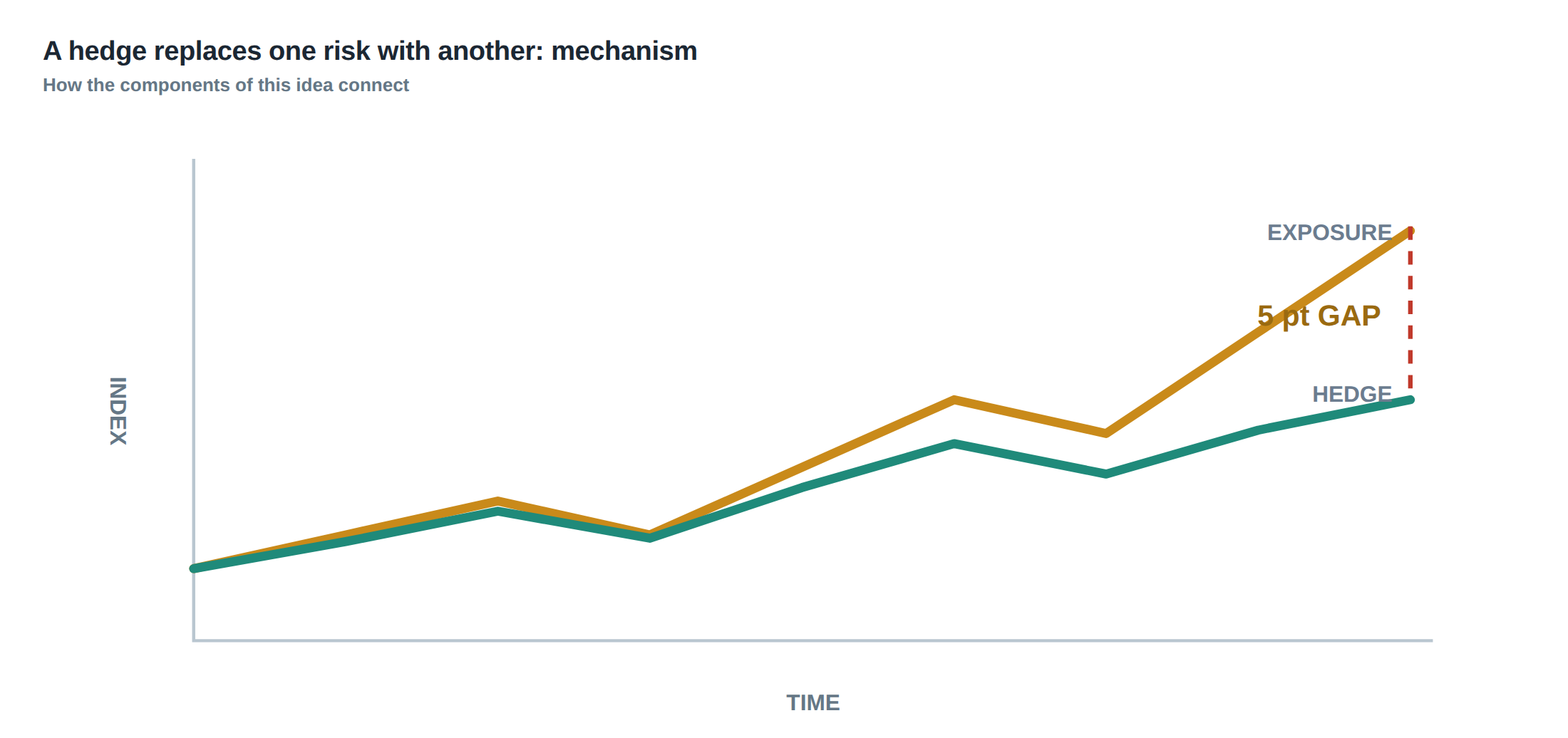
The phrase “a hedge replaces one risk with another” captures a paradox that every prop‑desk trader eventually confronts. When a position is exposed to a primary driver – for example, the price of a commodity future – the natural response is to offset that exposure with a correlated instrument, such as a calendar spread or a related index future. The intention is to neutralise the targeted factor, but the act of hedging inevitably creates a new set of exposures: basis risk, execution slippage, funding drag and the risk that the statistical relationship on which the hedge rests disintegrates when it matters most. In practice the hedge is never a perfect mirror; it is a statistical approximation that works well on average but can fail spectacularly in the tails. Understanding exactly what is being hedged, how the hedge ratio is estimated, and what residual risks remain is the first step towards disciplined risk management.

The core of the problem is that risk is a distribution, not a single point estimate. A hedge that removes the mean‑reverting component of the distribution may leave the variance – or worse, the skewness and kurtosis – largely untouched. Consequently, while the expected directional P&L may shrink, the probability of extreme loss can rise if the hedge introduces new sources of volatility. The trade‑off is therefore between reducing the targeted exposure and accepting additional layers of model, liquidity and operational risk.

In a fast‑moving strategy, latency and fill quality are often summarised by median values, but the true cost of a hedge is revealed in the tail of the latency distribution, in the frequency of stale orders, and in the loss profile when routing or cancellation behaves abnormally. The same principle applies to the hedge itself: the median basis may be small, yet the tail of basis widening can dominate the realised P&L during market stress.

How the mechanism works, step by step

The first step is to define the factor that drives the original exposure. In a crude‑oil long futures book, the factor is the spot price of WTI, proxied by the front‑month CL contract. The hedge is then chosen – for instance, a longer‑dated CL contract or an energy‑index future that historically moves 0.9 × the spot.

Next, the hedge ratio is estimated. A common approach is ordinary least‑squares regression of the target instrument’s returns against the proxy over a rolling window, yielding a slope (the hedge ratio) and a standard error that quantifies estimation uncertainty. The regression residuals provide a direct measure of basis risk.

The third step is to translate the ratio into an execution plan. If the target position is 10 000 barrels, and the estimated ratio is 0.78, the trader will sell 7 800 barrels worth of the proxy. The trade size is then adjusted for contract size, margin requirements and the expected financing cost of holding the hedge.

Finally, the hedge is monitored continuously. Divergence between the realised price path of the target and the hedge is recorded as a basis spread. When the spread exceeds a pre‑defined tolerance, the trader may unwind, roll, or augment the hedge. The monitoring loop also incorporates roll costs – the cost of moving from one contract month to the next – and financing costs, which can be significant for long‑dated proxies.

A worked example with real numbers

Consider a desk that holds a long exposure of 10 000 barrels of Brent crude, realised through the front‑month BZ futures contract. The desk wishes to hedge the price risk using the E-mini S&P 500 Energy Index future (ES‑EN), which historically exhibits a correlation of 0.85 with Brent returns.

Over the previous 252 trading days, a regression of daily log‑returns of BZ against ES‑EN yields a slope of 0.78 and a standard error of 0.04. The 95 % confidence interval for the hedge ratio is therefore 0.70 to 0.86, indicating modest estimation risk. The residual standard deviation – the basis risk – is 0.12 % of the notional per day.

Applying the point estimate, the desk sells 7 800 units of ES‑EN (0.78 × 10 000). Each ES‑EN contract represents 1 000 barrels of oil equivalent, so the trade consists of eight contracts (rounded to the nearest whole contract). The financing cost of the short position is 2.3 bp per annum, while the roll cost from the current contract to the next quarterly contract is 0.7 % of the notional, reflecting the typical term‑structure premium in energy futures.

During the first ten trading days, the basis – defined as the daily difference between the BZ P&L and the hedged P&L – remains within ±0.03 % of notional, well inside the pre‑set tolerance of 0.05 %. However, on day 12 a sudden supply shock in the North Sea causes Brent to jump 2 % while the ES‑EN index lags, widening the spread to 0.18 % of notional. The residual variance spikes, and the realised basis error for the ten‑day window rises to 0.15 % – three times the historical average.

If the desk had relied solely on the median basis, the hedge would appear satisfactory. The tail event, however, erodes 1.2 % of the portfolio’s value in a single day, a loss that exceeds the expected financing and roll costs combined. The example illustrates that the hedge reduces the average directional exposure but introduces a basis risk that can explode when the correlation breaks down.

Where it breaks in live markets

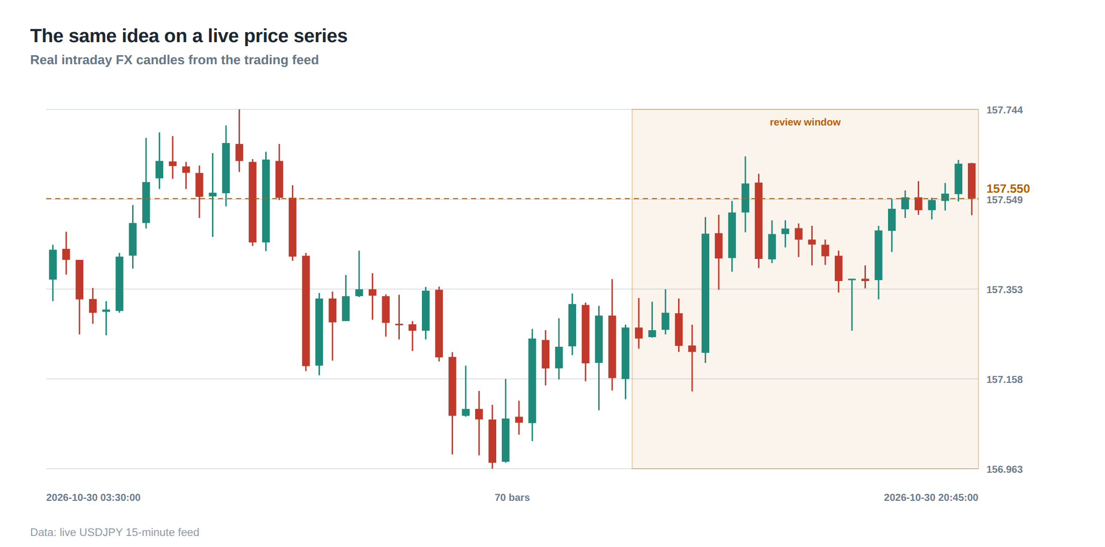
The statistical relationship that underpins any hedge is fragile. Correlations that hold in tranquil periods can collapse during crises, when market participants shift from arbitrage to flight‑to‑quality. In the example above, the proxy’s lag is a manifestation of differing liquidity pools: Brent futures trade on ICE, while the ES‑EN index is cleared through CME, each with its own order‑book depth and participant base. When a shock hits one venue, the other may not react synchronously, creating a transient but costly basis.

Liquidity risk compounds the problem. A hedge that is thinly traded can suffer from slippage when the desk attempts to scale the position quickly. Execution risk is amplified if the hedge must be rolled into a less liquid contract month; the price impact of the roll can dwarf the anticipated financing benefit.

Model risk is another hidden source of failure. The regression assumes linearity and stationarity, yet market dynamics are often non‑linear. Regime‑switching behaviour – for example, a sudden move from a backwardated to a contangoed term structure – can invalidate the hedge ratio overnight. If the desk does not re‑estimate the ratio frequently enough, the hedge can become mis‑aligned before the monitoring system flags the divergence.

Finally, operational risk – such as order‑routing failures, exchange outages, or settlement mismatches – can leave the hedge partially or wholly unexecuted. In a high‑frequency context, a missed hedge order during a latency spike may expose the desk to the full unhedged risk for several seconds, enough to generate a sizeable loss on a large notional.

The operating path, stage by stage

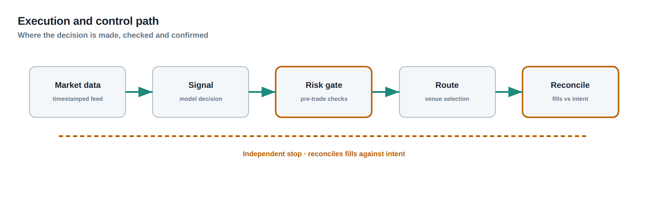
The hedge lifecycle can be broken into four distinct stages. The first stage is identification, where the risk factor is quantified and a proxy instrument is selected based on historical co‑movement and liquidity. The second stage is parameterisation, in which the hedge ratio and its confidence interval are calculated, and the financing and roll costs are projected.

The third stage is execution, where the hedge order is sent, monitored for fill quality, and any partial fills are reconciled against the target size. At this point, the desk must also allocate capital for margin and account for the financing drag of the short position.

The fourth stage is maintenance, encompassing real‑time tracking of the basis, periodic re‑estimation of the hedge ratio, and decision rules for rolling or unwinding. The maintenance loop is where the desk decides whether the hedge remains effective or whether to accept an incomplete hedge and adjust the underlying exposure accordingly.

Each stage introduces its own control points and failure modes, and the overall robustness of the hedge depends on how tightly the stages are coupled.

Controls that act before the damage

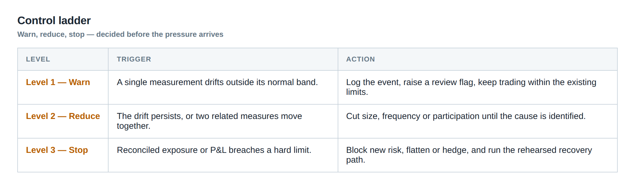
Preventive controls begin with a pre‑trade validation that checks the proxy’s liquidity, the expected slippage, and the alignment of contract expiry dates. The desk should enforce a minimum average daily volume threshold for the hedge instrument, and a maximum acceptable bid‑ask spread relative to the notional.

During order generation, a risk engine must verify that the notional of the hedge does not exceed the pre‑approved exposure limit, and that the projected financing cost stays within the budgeted range. A “what‑if” simulation of a rapid basis widening is run in parallel, generating a stress‑scenario P&L that must be below a pre‑set loss ceiling.

Execution controls include a latency guard that aborts the hedge order if the round‑trip time exceeds the 99th‑percentile of the historical latency distribution. A stale‑order filter discards any order that has been pending for longer than the median time‑to‑fill plus two standard deviations.

Finally, post‑trade reconciliation checks that the filled size matches the intended hedge ratio within the confidence interval. Any deviation triggers an automatic alert and a mandatory review before the hedge can be rolled forward. These layers of control aim to catch a problem before it propagates into the portfolio.

How to measure whether it is working

Effectiveness is assessed by comparing the realised variance of the hedged position against the variance of the unhedged exposure. A reduction of at least 60 % in daily variance is a typical benchmark for a well‑calibrated hedge. However, variance alone hides tail risk; therefore, the desk also tracks the 95 % and 99 % Value‑at‑Risk (VaR) of the hedged P&L.

Basis tracking is performed by calculating the cumulative spread between the target and hedge returns. The average absolute basis should remain below the tolerance set in the maintenance stage, while the standard deviation of the basis provides a measure of residual risk.

The cost side is measured by adding the financing drag, roll cost, and any execution slippage to the hedged P&L. If the total cost exceeds the reduction in risk (expressed in monetary terms), the hedge may be deemed uneconomical.

A further diagnostic is the hit‑rate of the confidence interval: the proportion of days where the realised hedge ratio falls within the pre‑computed 95 % confidence band. Consistently low hit‑rates indicate model miss‑specification or regime change, prompting a re‑estimation of the regression window.

The portfolio view

From a portfolio perspective, each hedge is a sub‑component of the overall risk budget. The aggregate basis risk of all hedged positions must be summed, taking into account correlation between the bases themselves. A common pitfall is to assume that diversifying across multiple hedges eliminates basis risk; in reality, many proxies share common drivers – for example, funding rates – and can move together in stress.

The desk therefore constructs a hedge‑adjusted covariance matrix, where each hedge’s residual exposure is represented as a separate factor. Portfolio optimisation then proceeds on this adjusted matrix, ensuring that the total VaR remains within the desk’s risk appetite after accounting for hedge costs.

Dynamic allocation between hedged and unhedged strategies can also be employed. When the confidence interval on the hedge ratio widens, the desk may reduce the size of the hedge and increase cash reserves, thereby limiting the potential loss from a basis breakout. Conversely, in periods of low volatility and tight basis, the hedge size can be expanded to capture additional risk‑adjusted return.

In sum, a hedge is not a static insurance policy but a dynamic position that must be managed, monitored, and re‑balanced in concert with the rest of the portfolio. Recognising that each mitigation step introduces its own risk class is essential to maintaining a resilient trading operation.

Do you have a systematic process in place to quantify and monitor the tail of the basis risk that your hedges generate?

About the research behind this lesson

Andrew Lo's lectures build risk analysis from return distributions and statistical measures, rather than treating one realised result as a complete description of risk.

Applied to this lesson: For a fast strategy, median latency or average fill quality is not enough. The review has to include tail delays, stale-order frequency and the loss distribution when cancellation or routing behaves abnormally.

Two live systems, one desk

PULSE-X — power-packed HFT: high-frequency momentum on XAUUSD and EURUSD. System details · Live account

NIC-X — ultra-low drawdown: displaced-print arbitrage for large capital. System details · Live account

Start now: leave your email and request a free trial — we will send the pricing, the connection route and the trial terms. Pricing

Join the market discussion: Telegram @squawklive

Source: Risk and Return

Educational content only. Trading leveraged products involves risk.