October 18, 2026

⛶

What this problem really is

Electronic markets are fundamentally queues that honour price‑time priority. Every new tick that arrives is inserted into a line whose position determines both the probability of execution and the expected profit from the spread. The value of a place in that line can be split into three components: the pure spread capture that would be earned if the order were filled immediately, the adverse‑selection cost that accrues while the order sits, and the optionality of remaining in line for a future favourable move. The latter two are time‑sensitive; the longer an order lingers, the more likely the queue position will be eroded by faster participants and the more the underlying price will drift away from the original signal. Consequently, the “speed” of a strategy is not a peripheral optimisation – it is an integral part of the economic model. A strategy that cannot react within the half‑life of its own signal simply trades a stale view of the market and erodes the optionality premium that the queue position once offered.

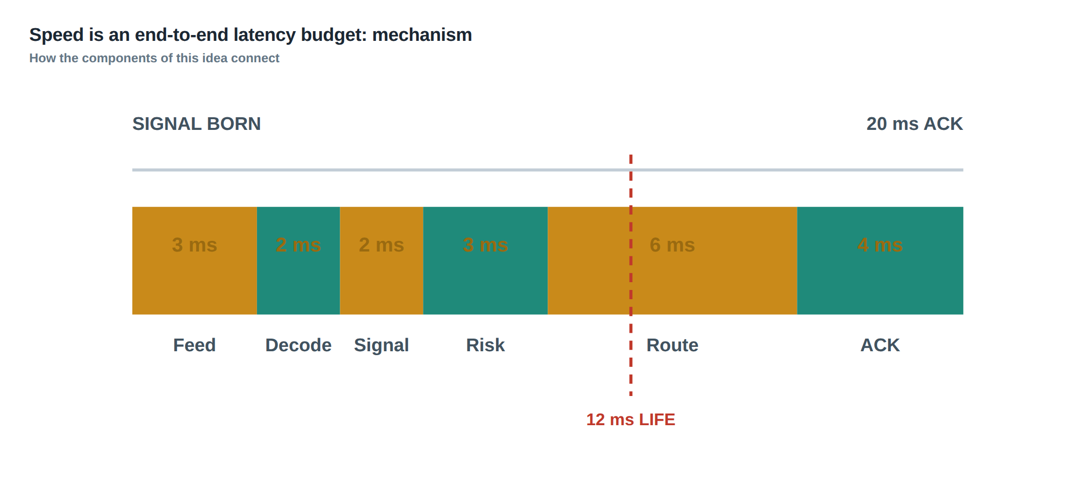
The latency budget therefore stretches from the instant a market data packet lands on the NIC to the moment an acknowledgement of the order’s fate is received back from the exchange. The slowest useful stage in that chain caps the overall usefulness of the signal. If any stage takes longer than the window in which the signal retains predictive power, the entire pipeline becomes a liability rather than an asset. The problem is therefore an end‑to‑end timing problem, not a collection of isolated micro‑optimisations.

How the mechanism works, step by step

The first stage is feed transit: the time taken for a market data packet to travel from the exchange’s data centre to the trader’s server. This is governed by physical distance, fibre or microwave path, and the quality of the exchange’s multicast implementation. Once the packet reaches the NIC, the kernel must copy it into user space, a step known as decoding. Modern low‑latency stacks use kernel bypass (DPDK, RDMA) to shave microseconds off this stage, but the cost is still measurable and varies with packet size and NIC load.

Decoded data then feeds the signal engine. Here the raw order‑book updates are transformed into a statistical indicator – for example a micro‑price imbalance or a short‑term momentum estimator. The computation itself may be a few arithmetic operations or a more complex machine‑learning inference; its duration is the “signal calculation” latency. The result is passed to a risk‑check module that validates size, price limits, position limits and any proprietary constraints.

If the risk check passes, the order is handed to the routing layer, which selects the destination (primary exchange, dark pool, internal crossing network) and formats the order according to the venue’s protocol. The order is then transmitted over a low‑latency link, typically a dedicated fibre pair. The exchange processes the order, places it in its internal queue, and eventually sends an acknowledgement (ack) or a fill notification back to the trader. The round‑trip from order submission to ack is the final leg of the latency budget.

Each of these stages adds both a deterministic component (e.g., known processing time) and a stochastic component (e.g., queuing delay on the NIC). The stochastic component is what creates tail latency and jitter, which are often far more damaging than the median latency because they can push the total response time beyond the signal’s half‑life on a non‑negligible fraction of trades.

A worked example with real numbers

Consider a mean‑reversion strategy that watches a 10‑tick micro‑price spread. Empirical analysis shows the spread’s autocorrelation decays to half its initial value after roughly twelve milliseconds; that is the signal half‑life. The strategy’s core computation – a weighted sum of the last three depth levels – takes two milliseconds on the current hardware configuration.

The feed transit from the exchange’s data centre to the firm’s colocation rack is 0.8 ms (median) with a 99th‑percentile of 1.3 ms. Decoding the multicast packet, using a zero‑copy kernel‑bypass library, adds 0.4 ms median and 0.7 ms at the 99th percentile. The risk‑check logic, which includes a real‑time VaR screen, consumes 0.3 ms median, 0.5 ms tail. Routing the order to the exchange’s matching engine adds another 0.6 ms median, 1.0 ms tail, while the exchange’s internal processing and ack generation contribute 1.5 ms median, 3.2 ms tail.

Summing the medians gives a total end‑to‑end latency of 5.6 ms, comfortably within the twelve‑millisecond half‑life. However, the 99th‑percentile tail adds up to 7.7 ms, still below the half‑life but leaving little margin for network jitter or occasional spikes in exchange load. If the routing layer were to experience a brief congestion episode that adds a further 5 ms to the tail, the total 99th‑percentile latency would rise to 12.7 ms, exceeding the signal’s useful window. In that scenario the two‑millisecond signal calculation provides little value; the order would arrive after the market has already moved away from the favourable price, and the optionality premium of the queue position would be largely gone.

The example illustrates that improving a single stage (e.g., shaving the signal calculation from 2 ms to 1 ms) does not guarantee a net gain unless the slowest stage is also reduced. The end‑to‑end budget is only as strong as its weakest link.

Where it breaks in live markets

In production, the latency budget is constantly assaulted by external and internal disturbances. Network congestion, especially on shared fibre routes, can produce occasional spikes that inflate the feed transit tail far beyond the median. Exchange‑level events – such as a sudden surge in order flow, a software upgrade, or a protective throttling mechanism – can increase the processing and ack latency dramatically for a few seconds.

Within the firm, CPU pre‑emptions, garbage‑collection pauses in managed runtimes, or contention on shared memory structures can introduce jitter that is hard to predict from bench‑marks. Even the most carefully engineered kernel‑bypass stack can suffer from NIC driver bugs that manifest only under high packet rates, leading to packet loss and retransmission delays.

When any of these factors pushes the total latency beyond the signal half‑life, the strategy’s edge evaporates. The order may still be filled, but at a price that no longer reflects the original predictive signal, turning a potential profit into an adverse‑selection loss. Moreover, because the market is a price‑time priority queue, a delayed order can also displace later orders that would have been more valuable, effectively eroding the optionality of the entire queue position.

The operating path, stage by stage

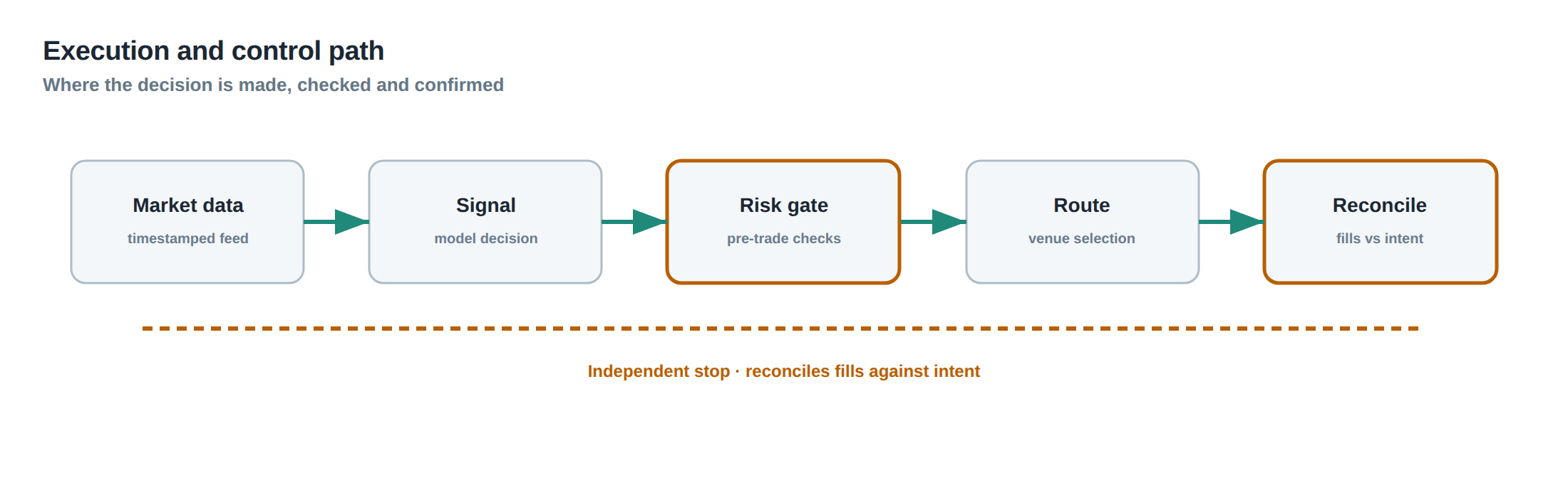
The end‑to‑end path can be visualised as a linear chain of stages, each with its own latency distribution. The first link is the market‑data feed, travelling over a physical medium that imposes a propagation delay proportional to distance; the second link is the NIC and its driver, which must move the packet from hardware buffers to user space. The third link is the decoding and deserialization routine, which transforms binary protocol fields into an in‑memory order‑book representation.

The fourth link is the signal engine, where the statistical model processes the refreshed book. The fifth link is the risk‑check module, which may involve look‑ups in position books and real‑time market‑risk tables. The sixth link is the order router, which selects the destination venue, formats the order, and hands it to the transmission stack. The seventh link is the outbound network path to the exchange, again subject to propagation and queuing delays. Finally, the eighth link is the exchange’s internal matching engine and the return ack path.

At each link, both the median latency and the tail latency matter. The median tells you the typical performance; the tail tells you how often you will breach the signal half‑life. Jitter – the variability between successive measurements – is a proxy for the tail: high jitter usually indicates a heavy tail. Understanding the distribution at each stage allows you to allocate optimisation effort where it will move the overall 99th‑percentile the most.

Controls that act before the damage

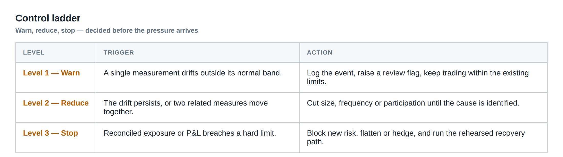
A robust latency‑budget framework includes proactive controls that prevent a slow path from ever reaching the market. First, clock synchronisation must be treated as part of the measurement system. Using a disciplined PTP (Precision Time Protocol) grandmaster and hardware timestamping on the NIC ensures that timestamps attached to incoming market data and outgoing acknowledgements are comparable across the whole chain. Without accurate clocks, latency measurements become noisy and can mask true tail events.

Second, a pre‑trade gating mechanism can abort the pipeline if any intermediate stage exceeds a configurable threshold. For example, if the signal calculation takes longer than four milliseconds, the order can be dropped before it reaches the risk engine. Similarly, a “deadline” timer can be attached to the routing stage; if the order has not been transmitted within six milliseconds of the original data‑arrival timestamp, it is discarded.

Third, adaptive load‑shedding at the NIC level can drop lower‑priority packets when the inbound rate exceeds a safe threshold, preserving headroom for the most latency‑sensitive feeds. Finally, continuous health‑checks – such as monitoring the 99th‑percentile latency of each stage and raising alerts when it drifts upward – allow the operations team to intervene before the degradation becomes systematic.

These controls act upstream of the market, preventing a slow order from ever entering the exchange’s queue and thereby protecting the optionality premium that the strategy seeks to capture.

How to measure whether it is working

Measurement must be end‑to‑end, not per‑stage in isolation. The most reliable method is to embed a unique identifier in each market‑data packet (e.g., a sequence number) and echo it back in the order acknowledgement. By recording the timestamp at the moment the packet is received (hardware‑timestamped on the NIC) and the timestamp when the ack is received, you obtain the full round‑trip latency for that specific event.

Collect these measurements continuously and compute not only the median but also the 95th, 99th and 99.9th percentiles. Plot the latency distribution over rolling windows to detect drift. Jitter can be quantified as the standard deviation of the inter‑arrival latency differences. Correlate latency spikes with external events (network alerts, exchange status messages) to identify root causes.

A further sanity check is to compare the observed latency distribution against the signal half‑life derived from historical back‑testing. If the 99th‑percentile consistently exceeds the half‑life, the strategy is operating in a regime where most trades are stale. In that case, the latency budget must be tightened or the signal horizon lengthened.

Regular audits of clock synchronisation accuracy – for instance, measuring the offset between the local PTP clock and a GPS reference – are also essential, because a drift of even a few microseconds can bias the latency histogram and hide tail events.

The portfolio view

When latency is viewed in isolation, it is tempting to optimise a single strategy without regard to the broader portfolio. In practice, a prop‑trading desk runs dozens of strategies that share the same hardware, network links and exchange connections. The latency budget of one strategy can therefore affect the tail latency of another through resource contention.

A portfolio‑wide latency model treats the total available “latency capacity” as a finite resource that must be allocated across strategies based on their signal half‑lives, expected turnover, and risk appetite. Strategies with ultra‑short half‑lives (sub‑millisecond) are given priority access to the fastest NIC queues and dedicated cores, while longer‑horizon strategies can tolerate higher tail latency and are placed on shared cores.

The operating budget is then expressed as a vector of per‑stage latency limits for each strategy, summed across the portfolio to stay within the physical limits of the infrastructure. Monitoring the aggregate tail latency ensures that no single strategy’s optimisation pushes the collective tail beyond the point where other strategies start to suffer. This holistic view prevents the “latency arms race” from degrading overall profitability and keeps the optionality value of queue positions intact across the desk.

Do you have a clear picture of which stage in your own end‑to‑end pipeline is the current bottleneck, and how it aligns with the half‑life of the signals you trade?

About the research behind this lesson

The seminar frames electronic markets as price-time-priority queues. It separates queue value into spread capture versus adverse-selection cost and the option value of retaining a place in line.

Applied to this lesson: An order lifetime therefore cannot be based on elapsed time alone: the system must reassess whether its queue position, expected spread and adverse-selection risk still justify keeping the order alive.

Explore PULSE: System details

PULSE live account: Verify the live account on FX Blue

Live chat and updates: Telegram @xtrskhft

Source: High-Frequency Trading and Modern Market Microstructure

Educational content only. Trading leveraged products involves risk.